
Randomness
Contents
6.2. Randomness#
6.2.1. Randomness#
We will use the numpy.random package to simulate randomness in Python.
This lecture will present various probability distributions and then use numpy.random to numerically verify some of the facts associated with them.
We import numpy as usual
import numpy as np
import matplotlib.pyplot as plt
%matplotlib inline
6.2.1.1. Probability#
Before we learn how to use Python to generate randomness, we should make sure that we all agree on some basic concepts of probability.
To think about the probability of some event occurring, we must understand what possible events could occur – mathematicians refer to this as the event space.
Some examples are
For a coin flip, the coin could either come up heads, tails, or land on its side.
The inches of rain falling in a certain location on a given day could be any real number between 0 and \( \infty \).
The change in an S&P500 stock price could be any real number between \( - \) opening price and \( \infty \).
An individual’s employment status tomorrow could either be employed or unemployed.
And the list goes on…
Notice that in some of these cases, the event space can be counted (coin flip and employment status) while in others, the event space cannot be counted (rain and stock prices).
We refer to random variables with countable event spaces as discrete random variables and random variables with uncountable event spaces as continuous random variables.
We then call certain numbers ‘probabilities’ and associate them with events from the event space.
The following is true about probabilities.
The probability of any event must be greater than or equal to 0.
The probability of all events from the event space must sum (or integrate) to 1.
If two events cannot occur at same time, then the probability that at least one of them occurs is the sum of the probabilities that each event occurs (known as independence).
We won’t rely on these for much of what we learn in this class, but occasionally, these facts will help us reason through what is happening.
6.2.1.2. Simulating Randomness in Python#
One of the most basic random numbers is a variable that has equal probability of being any value between 0 and 1.
You may have previously learned about this probability distribution as the Uniform(0, 1).
Let’s dive into generating some random numbers.
Run the code below multiple times and see what numbers you get.
np.random.rand()
0.7861231768856889
We can also generate arrays of random numbers.
np.random.rand(25)
array([0.80741591, 0.2414606 , 0.84430431, 0.66926319, 0.3655989 ,
       0.65405617, 0.62557491, 0.53152612, 0.28019645, 0.35207087,
       0.73278887, 0.12497625, 0.06393882, 0.3274459 , 0.52779755,
       0.89017999, 0.46144369, 0.6994162 , 0.22780065, 0.09016095,
       0.62091438, 0.79016224, 0.44779656, 0.10708325, 0.00984452])
np.random.rand(5, 5)
array([[0.01523257, 0.53493136, 0.93989972, 0.06885106, 0.26380146],
       [0.83308775, 0.45212772, 0.50914628, 0.28005659, 0.4640297 ],
       [0.03546809, 0.35908938, 0.71130438, 0.98707699, 0.06626503],
       [0.6114508 , 0.55178832, 0.93122069, 0.1212634 , 0.63745596],
       [0.50782802, 0.20273609, 0.42801359, 0.29403367, 0.34484808]])
np.random.rand(2, 3, 4)
array([[[0.80654196, 0.33543474, 0.67812728, 0.10922672],
        [0.87563335, 0.59962314, 0.96866144, 0.54953366],
        [0.53313724, 0.70226717, 0.96371935, 0.86167311]],

       [[0.50909714, 0.07516694, 0.06580736, 0.5436356 ],
        [0.10754751, 0.59794248, 0.65163124, 0.87937045],
        [0.70196581, 0.18642059, 0.63469207, 0.8524823 ]]])
6.2.1.3. Why Do We Need Randomness?#
As economists and data scientists, we study complex systems.
These systems have inherent randomness, but they do not readily reveal their underlying distribution to us.
In cases where we face this difficulty, we turn to a set of tools known as Monte Carlo methods.
These methods effectively boil down to repeatedly simulating some event (or events) and looking at the outcome distribution.
This tool is used to inform decisions in search and rescue missions, election predictions, sports, and even by the Federal Reserve.
The reasons that Monte Carlo methods work is a mathematical theorem known as the Law of Large Numbers.
The Law of Large Numbers basically says that under relatively general conditions, the distribution of simulated outcomes will mimic the true distribution as the number of simulated events goes to infinity.
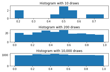
We already know how the uniform distribution looks, so let’s demonstrate the Law of Large Numbers by approximating the uniform distribution.
# Draw various numbers of uniform[0, 1] random variables
draws_10 = np.random.rand(10)
draws_200 = np.random.rand(200)
draws_10000 = np.random.rand(10_000)

# Plot their histograms
fig, ax = plt.subplots(3)

ax[0].set_title("Histogram with 10 draws")
ax[0].hist(draws_10)

ax[1].set_title("Histogram with 200 draws")
ax[1].hist(draws_200)

ax[2].set_title("Histogram with 10,000 draws")
ax[2].hist(draws_10000)

fig.tight_layout()
6.2.1.4. Continuous Distributions#
Recall that a continuous distribution is one where the value can take on an uncountable number of values.
It differs from a discrete distribution in that the events are not countable.
We can use simulation to learn things about continuous distributions as we did with discrete distributions.
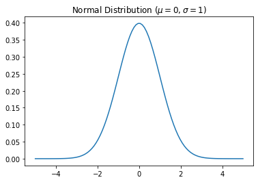
Let’s use simulation to study what is arguably the most commonly encountered distributions – the normal distribution.
The Normal (sometimes referred to as the Gaussian distribution) is bell-shaped and completely described by the mean and variance of that distribution.
The mean is often referred to as \( \mu \) and the variance as \( \sigma^2 \).
Let’s take a look at the normal distribution.
# scipy is an extension of numpy, and the stats
# subpackage has tools for working with various probability distributions
import scipy.stats as st

x = np.linspace(-5, 5, 100)

# NOTE: first argument to st.norm is mean, second is standard deviation sigma (not sigma^2)
pdf_x = st.norm(0.0, 1.0).pdf(x)

fig, ax = plt.subplots()

ax.set_title(r"Normal Distribution ($\mu = 0, \sigma = 1$)")
ax.plot(x, pdf_x)
[<matplotlib.lines.Line2D at 0x20a9ede1400>]
You can use the isf method to get the inverst cumulative density function of the distribution and recover the threshold associated with a particular probability mass in the tails
Here you passe the probability, say 5% and the function returns the threshold so there is exactly this probability mass to the right of it.
# right tail
st.norm(0.,1.).isf(0.05)
1.6448536269514729
# left tail
st.norm(0.,1.).isf(0.95)
-1.6448536269514722
And you can obvioulsy simulate as well
Here I simualte a standard normal vector with 3 rows and 4 columns
st.norm(0.,1.).rvs(size=(3,4))
array([[-1.94292854,  0.53350177, -0.95225937, -0.81668611],
       [ 0.41954983, -2.05398858, -1.25605238,  1.18249787],
       [ 0.01225393, -1.53787579, -0.89654655, -2.01561892]])
Here a column vector
st.norm(0.,1.).rvs(size=10)
array([-0.38103522, -1.88341677, -1.42194613, -0.07887213, -0.17482899,
        0.4912504 ,  0.02407146, -2.69009789, -1.08301844,  1.68147818])
You can also this to compute means (in the case of the normal is silly)
st.norm(0.,1.).mean()
0.0
st.norm(0.,1.).std()
1.0
But also higher order moments!
# kurtosis!
st.norm(0.,1.).moment(4)
3.0
6.2.1.5. Optional content: Discrete Distributions#
Sometimes we will encounter variables that can only take one of a few possible values.
We refer to this type of random variable as a discrete distribution.
For example, consider a small business loan company.
Imagine that the company’s loan requires a repayment of \( \\\)25,000 $ and must be repaid 1 year after the loan was made.
The company discounts the future at 5%.
Additionally, the loans made are repaid in full with 75% probability, while \( \\\)12,500 $ of loans is repaid with probability 20%, and no repayment with 5% probability.
How much would the small business loan company be willing to loan if they’d like to – on average – break even?
In this case, we can compute this by hand:
The amount repaid, on average, is: \( 0.75(25,000) + 0.2(12,500) + 0.05(0) = 21,250 \).
Since we’ll receive that amount in one year, we have to discount it: \( \frac{1}{1+0.05} 21,250 \approx 20238 \).
We can now verify by simulating the outcomes of many loans.
# You'll see why we call it `_slow` soon :)
def simulate_loan_repayments_slow(N, r=0.05, repayment_full=25_000.0,
                                  repayment_part=12_500.0):
    repayment_sims = np.zeros(N)
    for i in range(N):
        x = np.random.rand()  # Draw a random number

        # Full repayment 75% of time
        if x < 0.75:
            repaid = repayment_full
        elif x < 0.95:
            repaid = repayment_part
        else:
            repaid = 0.0

        repayment_sims[i] = (1 / (1 + r)) * repaid

    return repayment_sims

print(np.mean(simulate_loan_repayments_slow(25_000)))
20195.23809523809
6.2.1.5.1. Advanced content: The extreme benefits of Vectorized Computations#
The code above illustrates the concepts we were discussing but is much slower than necessary.
Below is a version of our function that uses numpy arrays to perform computations instead of only storing the values.
def simulate_loan_repayments(N, r=0.05, repayment_full=25_000.0,
                             repayment_part=12_500.0):
    """
    Simulate present value of N loans given values for discount rate and
    repayment values
    """
    random_numbers = np.random.rand(N)

    # start as 0 -- no repayment
    repayment_sims = np.zeros(N)

    # adjust for full and partial repayment
    partial = random_numbers <= 0.20
    repayment_sims[partial] = repayment_part

    full = ~partial & (random_numbers <= 0.95)
    repayment_sims[full] = repayment_full

    repayment_sims = (1 / (1 + r)) * repayment_sims

    return repayment_sims

np.mean(simulate_loan_repayments(25_000))
20240.476190476187
We’ll quickly demonstrate the time difference in running both function versions.
%timeit simulate_loan_repayments_slow(250_000)
117 ms ± 1.36 ms per loop (mean ± std. dev. of 7 runs, 10 loops each)
%timeit simulate_loan_repayments(250_000)
4.21 ms ± 81.8 µs per loop (mean ± std. dev. of 7 runs, 100 loops each)
The timings for my computer were 1114 ms for simulate_loan_repayments_slow and 4.2 ms for
simulate_loan_repayments.
This function is simple enough that both times are acceptable, but the 33x time difference could matter in a more complicated operation.
This illustrates a concept called vectorization, which is when computations operate on an entire array at a time.
In general, numpy code that is vectorized will perform better than numpy code that operates on one element at a time.