
Multi-factor models
import numpy as np
import pandas as pd
%matplotlib inline
import matplotlib.pyplot as plt
14.4. Multi-factor models#
Adding factors to proxy for the total wealth portfolio
According to the CAPM the Wealth portfolio is the tangency portfolio
The return on the wealth portfolio summarizes how Bad the times are
Assets that co-vary more with the market must earn higher returns
They pay poorly exactly when things are worse
What is the wealth portfolio? It is the portfolio that holds all assets in proportion to their value
We often use the equity market as a proxy for this, but that is not the CAPM
In a way that CAPM is untestable because it is impossible to construct the true wealth portfolio
The fact that we cannot really measure the returns of the total wealth protfolio gives us a reason to add other facts in additons to the returns to the equity market. Under this logic you add returns to other assets classes>
Real estate
Corporate debt
Human capital
Private equity
Venture Capital -…
So you get:
where \(a\) are the different asset classes.
Sometimes people refer to these other hard to trade assets as “background risks”, basically risks that are you are exposed to that are not capture by your financial assets
ICAPM: Intertemporal Capital Asset Pricing Model
Another way to rationalize additional factors is to realize that the premium and the volatiltiy of the market are time-varying.
This means that assets that allow you to hedge this investment opportunity set risk will be valuable
For example, an asset that pays well when the market is more/less volatile or one that pays well when the expected reutrns of market going froward are higher/lower
Under this logic, any strategy that is related to the market moments can also explain average returns on top of the marker beta
Sometimes people refer to the background risks discussed earlier in this framework as well. But in this case it is not about the moments of the market portfolio per se, but about correlation of the strategy with the background risks investors bear
The end result is the same
but now these are “Factors” and do no need to be components of the total wealth
but these factors must still be excess returns, i.e. they must be strategies based on financial assets that have price zero
APT: Arbitrage Pricing Theory
Yet another model that has exaclty the same prediction
but now the factors are motivated because the explain time-seires variation in realized return
the idea is that if you have enough factors you explain enough of the variaiton in the returns of an asset that if the betas do no explain the average reuturns than an arbitrage opportunity wouldd open up
So you can think of the first two moticaiton being more about “economic factors” while this one being abotu “fianncail factors”. The factors belong if they help you explain reuturs.
APT in the end is a very statistical model
How to work with multifactor models?
These models make less restrictive assumptions and predict that we will need additional factors beyond the market to “span” the tangency portfolio
What does “span” mean?
It is basically the same as before, but now we run a multivariate regression
\[R_{i,t}=\alpha_i+\beta_{mkt}R^{mkt}_t+\beta_1 Factor_1+\beta_2 Factor_2+\beta_3 Factor_3+....+\beta_n Factor_n+\epsilon_{i,t}\]As long as the factors are also excess returns, the time-series alpha test is still valid and indentical as before.
You can do single asset tests and simply use the alpha t-stat to test the model
Everything that we discussed with the hedging/tracking portfolios apply here as well, but now
where \((\beta_{mkt}R^{mkt}_t+\beta_1 Factor_1+\beta_2 Factor_2+\beta_3 Factor_3+....+\beta_n Factor_n)\) is the tracking portfolio
Which Multi-factor models?
It really depends on the application. Practicioners ofen use factor models with 10 or more factors becasue they are interested in peformance attibution.
You use the regression to see which factor explain some particular realized performance while not thinking to much about whether the factor there explains average returns.
This is a perferctly good use mulitfactor models. In this case you are not really thinking whether the factors help you span the tangency portfolio, but only if it help explain the realized reutrn of the strategy.
If you interesting in accounting for a fund/strategy/stock averagare return you have look for factors that help you span the tangency portfolio, i.e. facots that generate high sharpe ratios.
In the academic world and also in a good chunk of practicioners people use the following factor models
Fama French 3 factor model:
Carhart 4 factor model:
Fama French 5 factor model:
Fama French 5 factor model + Momentum:
Where :
HmL is the value strategy that buys high book to market firms and sell low book to market firms
SmB is a size strategy that buys firms with low market capitalization and sell firms with high market capitalizations
WmL is the momentum strategy that buy stocks that did well in the last 12 months and short the ones that did poorly
RmW is the strategy that buys firms with high gross proftiability and sell firms with low gross profitability
CmA is the strategy that buys firms that are investing little (low CAPEX) and sell firms that are investing a lot (high CAPEX)
Three applications to evalauting asset managers
We will do this in three steps
Get time-series of the factors in our factor model and the risk-free rate
For each application get the time-series return data of the asset being evaluated
Merge with factor series
Convert the returns of the asset being evaluate to excess returns
Run a time-series regression of the asset excess returns on the relevant factors
Factors for our factor model
We will start by dowloading he Five factors from Fama Frency 5 factors model plus the momentum factor which is in separate data set
We of course could have constructed them ourselves as well, but this is obviously faster and less error prone
from datetime import datetime
import pandas_datareader.data as web
start = datetime(1926, 1, 1)
ds = web.DataReader('F-F_Research_Data_5_Factors_2x3', 'famafrench',start=start)
dff5=ds[0][:'2021-3']
dff5
ds = web.DataReader('F-F_Momentum_Factor', 'famafrench',start=start)
dmom=ds[0][:'2021-3']
dmom
dff6=dff5.merge(dmom,left_index=True,right_index=True,how='inner')
dff6
| Mkt-RF | SMB | HML | RMW | CMA | RF | Mom | |
|---|---|---|---|---|---|---|---|
| Date | |||||||
| 1963-07 | -0.39 | -0.45 | -0.94 | 0.66 | -1.15 | 0.27 | 1.00 |
| 1963-08 | 5.07 | -0.82 | 1.82 | 0.40 | -0.40 | 0.25 | 1.03 |
| 1963-09 | -1.57 | -0.48 | 0.17 | -0.76 | 0.24 | 0.27 | 0.16 |
| 1963-10 | 2.53 | -1.30 | -0.04 | 2.75 | -2.24 | 0.29 | 3.14 |
| 1963-11 | -0.85 | -0.85 | 1.70 | -0.45 | 2.22 | 0.27 | -0.75 |
| ... | ... | ... | ... | ... | ... | ... | ... |
| 2020-11 | 12.47 | 6.75 | 2.11 | -2.78 | 1.05 | 0.01 | -12.25 |
| 2020-12 | 4.63 | 4.67 | -1.36 | -2.15 | 0.00 | 0.01 | -2.42 |
| 2021-01 | -0.03 | 6.88 | 2.85 | -3.33 | 4.68 | 0.00 | 4.37 |
| 2021-02 | 2.78 | 4.51 | 7.08 | 0.09 | -1.97 | 0.00 | -7.68 |
| 2021-03 | 3.09 | -0.98 | 7.40 | 6.43 | 3.44 | 0.00 | -5.83 |
693 rows × 7 columns
Aplication 1: Performance evaluation of Berkshire Hathaway
How much of WB performance can be explained by his exposure to the differnet risk factors?
How much of WB performance is due to his ability to buy good business for cheap?
Getting the Data
We will do the data at monthly frequency.
While daily data is helpful in estiamting betas we have do be mindful of liqudiity effects, for example bid-ask bounces
One could do daily and add lagged returns as a way to deal with this
import wrds
import psycopg2
from codesnippets import get_returns
conn=wrds.Connection()

def get_returns(tickers,conn,startdate,enddate,variable='ret'):
    ticker=tickers[0]
    df = conn.raw_sql("""
                          select a.permno, b.ncusip, b.ticker, a.date, b.shrcd,
                          a.ret, a.vol, a.shrout, a.prc, a.cfacpr, a.cfacshr,a.retx
                          from crsp.msf as a
                          left join crsp.msenames as b
                          on a.permno=b.permno
                          and b.namedt<=a.date
                          and a.date<=b.nameendt
                          where a.date between '"""+ startdate+"""'  and '"""+ enddate+
                          """' and  b.ticker='"""+ticker+"'")
    # and b.shrcd between 10 and 11
    # and b.exchcd between 1 and 3

    df.set_index(['date','permno'],inplace=True)
    df=df[variable].unstack()
    return df
Enter your WRDS username [Alan.Moreira]: moreira5
Enter your password: ···········
WRDS recommends setting up a .pgpass file.
You can find more info here:
https://www.postgresql.org/docs/9.5/static/libpq-pgpass.html.
Loading library list...
Done
df=get_returns(['BRK'],conn,'1/1/1960','1/1/2022',variable='prc')
df.abs().plot()
<AxesSubplot:xlabel='date'>
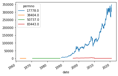
Berkshire seems to have multiple securities issue over time
We will simply use the blue series which matches wha tI see in google, but you could think about piecing toghether the blue and the green to expand the sample. But one would have to read in detail to see what happened and if that really makes sense
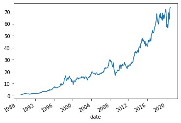
df=get_returns(['BRK'],conn,'1/1/1960','1/1/2022',variable='ret')
(df[17778.0]+1).cumprod().plot()
<AxesSubplot:xlabel='date'>
Lets now merge with the factors
Firs note that they are both monthy bu the factors index is period type while the Berkshire index is date time
dff6.index
PeriodIndex(['1963-07', '1963-08', '1963-09', '1963-10', '1963-11', '1963-12',
             '1964-01', '1964-02', '1964-03', '1964-04',
             ...
             '2020-06', '2020-07', '2020-08', '2020-09', '2020-10', '2020-11',
             '2020-12', '2021-01', '2021-02', '2021-03'],
            dtype='period[M]', name='Date', length=693, freq='M')
df.index
DatetimeIndex(['1962-08-31', '1962-09-28', '1962-10-31', '1962-11-30',
               '1962-12-31', '1963-01-31', '1963-02-28', '1963-03-29',
               '1963-04-30', '1963-05-31',
               ...
               '2020-03-31', '2020-04-30', '2020-05-29', '2020-06-30',
               '2020-07-31', '2020-08-31', '2020-09-30', '2020-10-30',
               '2020-11-30', '2020-12-31'],
              dtype='datetime64[ns]', name='date', length=644, freq=None)
We can deal with this by converting either the df dataframe to period or the dff6 dataframe to datetime
df[17778.0].to_period("M").tail()
date
2020-08    0.115550
2020-09   -0.023077
2020-10   -0.054690
2020-11    0.136159
2020-12    0.012008
Freq: M, Name: 17778.0, dtype: float64
dff6.to_timestamp('M').tail()
| Mkt-RF | SMB | HML | RMW | CMA | RF | Mom | |
|---|---|---|---|---|---|---|---|
| Date | |||||||
| 2020-11-30 | 12.47 | 6.75 | 2.11 | -2.78 | 1.05 | 0.01 | -12.25 |
| 2020-12-31 | 4.63 | 4.67 | -1.36 | -2.15 | 0.00 | 0.01 | -2.42 |
| 2021-01-31 | -0.03 | 6.88 | 2.85 | -3.33 | 4.68 | 0.00 | 4.37 |
| 2021-02-28 | 2.78 | 4.51 | 7.08 | 0.09 | -1.97 | 0.00 | -7.68 |
| 2021-03-31 | 3.09 | -0.98 | 7.40 | 6.43 | 3.44 | 0.00 | -5.83 |
Here I will use the first method
df=(dff6/100).merge(df[17778.0].to_period("M"),left_index=True,right_index=True,how='inner').dropna(how='any')
df.rename(columns={17778:'BRK'},inplace=True)
df
| Mkt-RF | SMB | HML | RMW | CMA | RF | Mom | BRK | |
|---|---|---|---|---|---|---|---|---|
| 1988-11 | -0.0229 | -0.0166 | 0.0130 | -0.0028 | 0.0160 | 0.0057 | 0.0042 | -0.005291 |
| 1988-12 | 0.0149 | 0.0201 | -0.0154 | 0.0063 | -0.0037 | 0.0063 | 0.0042 | 0.000000 |
| 1989-01 | 0.0610 | -0.0223 | 0.0049 | -0.0103 | 0.0016 | 0.0055 | -0.0014 | 0.047872 |
| 1989-02 | -0.0225 | 0.0267 | 0.0090 | -0.0081 | 0.0190 | 0.0061 | 0.0094 | -0.040609 |
| 1989-03 | 0.0157 | 0.0077 | 0.0047 | 0.0000 | 0.0079 | 0.0067 | 0.0356 | 0.047619 |
| ... | ... | ... | ... | ... | ... | ... | ... | ... |
| 2020-08 | 0.0763 | -0.0094 | -0.0294 | 0.0427 | -0.0144 | 0.0001 | 0.0051 | 0.115550 |
| 2020-09 | -0.0363 | 0.0007 | -0.0251 | -0.0115 | -0.0177 | 0.0001 | 0.0305 | -0.023077 |
| 2020-10 | -0.0210 | 0.0476 | 0.0403 | -0.0060 | -0.0053 | 0.0001 | -0.0303 | -0.054690 |
| 2020-11 | 0.1247 | 0.0675 | 0.0211 | -0.0278 | 0.0105 | 0.0001 | -0.1225 | 0.136159 |
| 2020-12 | 0.0463 | 0.0467 | -0.0136 | -0.0215 | 0.0000 | 0.0001 | -0.0242 | 0.012008 |
386 rows × 8 columns
df.BRK=df.BRK-df.RF
Start with the CAPM
import statsmodels.api as sm
temp=df.copy()
x= sm.add_constant(temp['Mkt-RF'])
y= temp['BRK']
results= sm.OLS(y,x).fit()
results.summary()
| Dep. Variable: | BRK | R-squared: | 0.212 |
|---|---|---|---|
| Model: | OLS | Adj. R-squared: | 0.210 |
| Method: | Least Squares | F-statistic: | 103.6 |
| Date: | Tue, 04 May 2021 | Prob (F-statistic): | 1.06e-21 |
| Time: | 09:25:48 | Log-Likelihood: | 592.00 |
| No. Observations: | 386 | AIC: | -1180. |
| Df Residuals: | 384 | BIC: | -1172. |
| Df Model: | 1 | ||
| Covariance Type: | nonrobust |
| coef | std err | t | P>|t| | [0.025 | 0.975] | |
|---|---|---|---|---|---|---|
| const | 0.0060 | 0.003 | 2.210 | 0.028 | 0.001 | 0.011 |
| Mkt-RF | 0.6236 | 0.061 | 10.178 | 0.000 | 0.503 | 0.744 |
| Omnibus: | 83.751 | Durbin-Watson: | 2.060 |
|---|---|---|---|
| Prob(Omnibus): | 0.000 | Jarque-Bera (JB): | 261.498 |
| Skew: | 0.974 | Prob(JB): | 1.65e-57 |
| Kurtosis: | 6.530 | Cond. No. | 23.0 |
Notes:
[1] Standard Errors assume that the covariance matrix of the errors is correctly specified.
results.params[0]*12
0.07164885662375453
Market beta of about 0.6 and alpha of 7% per year!
Six factor model
temp=df.copy()
x= sm.add_constant(temp.drop(['BRK','RF'],axis=1))
y= temp['BRK']
results= sm.OLS(y,x).fit()
results.summary()
| Dep. Variable: | BRK | R-squared: | 0.348 |
|---|---|---|---|
| Model: | OLS | Adj. R-squared: | 0.338 |
| Method: | Least Squares | F-statistic: | 33.74 |
| Date: | Tue, 04 May 2021 | Prob (F-statistic): | 1.35e-32 |
| Time: | 09:26:02 | Log-Likelihood: | 628.50 |
| No. Observations: | 386 | AIC: | -1243. |
| Df Residuals: | 379 | BIC: | -1215. |
| Df Model: | 6 | ||
| Covariance Type: | nonrobust |
| coef | std err | t | P>|t| | [0.025 | 0.975] | |
|---|---|---|---|---|---|---|
| const | 0.0046 | 0.003 | 1.774 | 0.077 | -0.001 | 0.010 |
| Mkt-RF | 0.7599 | 0.067 | 11.357 | 0.000 | 0.628 | 0.892 |
| SMB | -0.3946 | 0.091 | -4.316 | 0.000 | -0.574 | -0.215 |
| HML | 0.4836 | 0.118 | 4.091 | 0.000 | 0.251 | 0.716 |
| RMW | 0.2687 | 0.121 | 2.214 | 0.027 | 0.030 | 0.507 |
| CMA | -0.1286 | 0.172 | -0.749 | 0.454 | -0.466 | 0.209 |
| Mom | -0.0077 | 0.057 | -0.135 | 0.892 | -0.119 | 0.104 |
| Omnibus: | 89.527 | Durbin-Watson: | 2.143 |
|---|---|---|---|
| Prob(Omnibus): | 0.000 | Jarque-Bera (JB): | 237.376 |
| Skew: | 1.105 | Prob(JB): | 2.85e-52 |
| Kurtosis: | 6.143 | Cond. No. | 80.7 |
Notes:
[1] Standard Errors assume that the covariance matrix of the errors is correctly specified.
print(results.params[0]*12)
0.055415983696528254
What do we learn about Warren Investment style?
What do we learn about Warren specific stock picking skills?
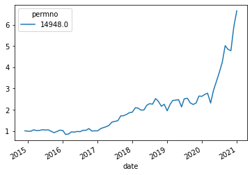
Aplication 2: Does Cathie Wood has some secret sauce? Performance evalaution of ARKK
df=get_returns(['ARKK'],conn,'1/1/1960','1/1/2022',variable='ret')
(df+1).cumprod().plot()
<AxesSubplot:xlabel='date'>
df=(dff6/100).merge(df.to_period("M"),left_index=True,right_index=True,how='inner').dropna(how='any')
df.rename(columns={14948.0:'ARKK'},inplace=True)
df.ARKK=df.ARKK-df.RF
temp=df.copy()
x= sm.add_constant(temp['Mkt-RF'])
y= temp['ARKK']
results= sm.OLS(y,x).fit()
results.summary()
| Dep. Variable: | ARKK | R-squared: | 0.691 |
|---|---|---|---|
| Model: | OLS | Adj. R-squared: | 0.687 |
| Method: | Least Squares | F-statistic: | 160.9 |
| Date: | Tue, 04 May 2021 | Prob (F-statistic): | 4.98e-20 |
| Time: | 09:28:12 | Log-Likelihood: | 120.93 |
| No. Observations: | 74 | AIC: | -237.9 |
| Df Residuals: | 72 | BIC: | -233.2 |
| Df Model: | 1 | ||
| Covariance Type: | nonrobust |
| coef | std err | t | P>|t| | [0.025 | 0.975] | |
|---|---|---|---|---|---|---|
| const | 0.0115 | 0.006 | 2.016 | 0.048 | 0.000 | 0.023 |
| Mkt-RF | 1.5768 | 0.124 | 12.684 | 0.000 | 1.329 | 1.825 |
| Omnibus: | 4.334 | Durbin-Watson: | 1.974 |
|---|---|---|---|
| Prob(Omnibus): | 0.115 | Jarque-Bera (JB): | 3.484 |
| Skew: | 0.465 | Prob(JB): | 0.175 |
| Kurtosis: | 3.516 | Cond. No. | 22.3 |
Notes:
[1] Standard Errors assume that the covariance matrix of the errors is correctly specified.
print(results.params[0]*12)
0.1385421007873513
temp=df.copy()
x= sm.add_constant(temp.drop(['ARKK','RF'],axis=1))
y= temp['ARKK']
results= sm.OLS(y,x).fit()
results.summary()
| Dep. Variable: | ARKK | R-squared: | 0.818 |
|---|---|---|---|
| Model: | OLS | Adj. R-squared: | 0.802 |
| Method: | Least Squares | F-statistic: | 50.21 |
| Date: | Tue, 04 May 2021 | Prob (F-statistic): | 6.69e-23 |
| Time: | 09:28:44 | Log-Likelihood: | 140.55 |
| No. Observations: | 74 | AIC: | -267.1 |
| Df Residuals: | 67 | BIC: | -251.0 |
| Df Model: | 6 | ||
| Covariance Type: | nonrobust |
| coef | std err | t | P>|t| | [0.025 | 0.975] | |
|---|---|---|---|---|---|---|
| const | 0.0059 | 0.005 | 1.234 | 0.221 | -0.004 | 0.015 |
| Mkt-RF | 1.3860 | 0.126 | 11.009 | 0.000 | 1.135 | 1.637 |
| SMB | 0.5065 | 0.210 | 2.410 | 0.019 | 0.087 | 0.926 |
| HML | -0.8120 | 0.200 | -4.067 | 0.000 | -1.211 | -0.413 |
| RMW | -0.1642 | 0.326 | -0.504 | 0.616 | -0.815 | 0.487 |
| CMA | -0.9219 | 0.351 | -2.624 | 0.011 | -1.623 | -0.221 |
| Mom | -0.2654 | 0.152 | -1.747 | 0.085 | -0.569 | 0.038 |
| Omnibus: | 10.376 | Durbin-Watson: | 2.119 |
|---|---|---|---|
| Prob(Omnibus): | 0.006 | Jarque-Bera (JB): | 10.331 |
| Skew: | 0.806 | Prob(JB): | 0.00571 |
| Kurtosis: | 3.866 | Cond. No. | 83.6 |
Notes:
[1] Standard Errors assume that the covariance matrix of the errors is correctly specified.
print(results.params[0]*12)
0.0704257048781867
What do we learn about Cathie Wood investment style?
What do we learn about Cathie Wook investment skills?
How do you think about the R-squared? Is a large Rsquared good or bad in this case?
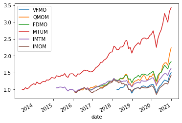
Application 3: what is a good Momentum ETF?
names=['VFMO','QMOM','FDMO','MTUM','IMTM','IMOM']
dmom=get_returns([names[0]],conn,'1/1/1960','1/1/2022')
for n in names[1:]:
    df=get_returns([n],conn,'1/1/1960','1/1/2022')
    dmom=dmom.merge(df,left_index=True,right_index=True,how='outer')
dmom.columns=names
(dmom+1).cumprod().plot()
<AxesSubplot:xlabel='date'>
# lets merge
df=(dff6/100).merge(dmom.to_period("M"),left_index=True,right_index=True,how='inner')
# lets conver to excess returns
df[names]=df[names].subtract(df['RF'],axis=0)
temp.columns
Index(['Mkt-RF', 'SMB', 'HML', 'RMW', 'CMA', 'RF', 'Mom   ', 'VFMO', 'QMOM',
       'FDMO', 'MTUM', 'IMTM', 'IMOM'],
      dtype='object')
temp=df.copy()
x= sm.add_constant(temp[['Mkt-RF','Mom   ']])
results=pd.DataFrame([],index=[],columns=names)
for n in names:
    y= temp[n]
    res= sm.OLS(y,x,missing='drop').fit()
    results.at['alpha',n]=res.params[0]
    results.at['t(alpha)',n]=res.tvalues[0]
    results.at['betamkt',n]=res.params[1]
    results.at['t(betamkt)',n]=res.tvalues[1]
    results.at['betamom',n]=res.params[2]
    results.at['t(betamom)',n]=res.tvalues[2]
    results.at['R-squared',n]=res.rsquared
    results.at['indio risk',n]=res.resid.std()*12**0.5
    results.at['sample size',n]=res.nobs
results
| VFMO | QMOM | FDMO | MTUM | IMTM | IMOM | |
|---|---|---|---|---|---|---|
| alpha | -0.001458 | -0.002718 | -0.002354 | 0.001112 | -0.002008 | -0.005894 |
| t(alpha) | -0.430959 | -0.63581 | -1.664363 | 0.869311 | -0.847557 | -1.459713 |
| betamkt | 1.132283 | 1.39176 | 1.024135 | 1.00483 | 0.761741 | 0.958616 |
| t(betamkt) | 16.762846 | 13.753471 | 31.996319 | 31.597999 | 13.558808 | 10.029335 |
| betamom | 0.186237 | 0.394746 | 0.254752 | 0.345416 | 0.09699 | 0.15187 |
| t(betamom) | 2.178768 | 3.281823 | 6.461063 | 9.626601 | 1.568105 | 1.336749 |
| R-squared | 0.917845 | 0.782982 | 0.960205 | 0.919332 | 0.756383 | 0.674357 |
| indio risk | 0.064076 | 0.107838 | 0.032342 | 0.039782 | 0.065174 | 0.101857 |
| sample size | 34.0 | 60.0 | 51.0 | 92.0 | 71.0 | 60.0 |
what do you conclude?
Which ETF would you pick?
How to think about the alpha here?
How do you think about the R-squared? Is a large Rsquared good or bad in this case?
How do you account for the differnece in market betas when investing?