# start by loading data on the returns of the market portfolio and the risk-free rate
import pandas as pd
import numpy as np
import matplotlib.pyplot as plt
%matplotlib inline

6.5. Dat APIs

• Pandas has an eco-system of APIs that allow you to get data from the web directly into a pandas dataframe

FRED

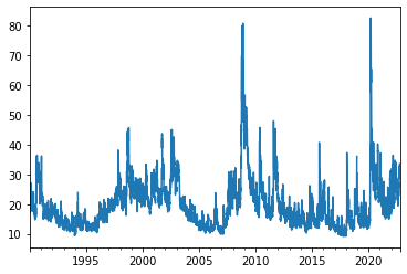
• Here we will look at one API that gets macro and financial data from the Federal Reserve Bank of St louis

• Lots and lots of data!

  https://fred.stlouisfed.org/categories

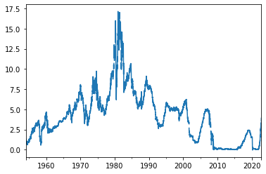
• For example the yield on the three month treasury bill

  https://fred.stlouisfed.org/series/DTB3

• you will also need to apply for an API key here

  https://research.stlouisfed.org/docs/api/api_key.html

• once you have it you use it to do this:

#!pip install fredapi
from fredapi import Fred
fred = Fred(api_key='f9207136b3333d7cf92c07273f6f5530')
data = fred.get_series('DTB3')
data.plot()

<AxesSubplot:>

data = fred.get_series('VIXCLS')
data.plot()

<AxesSubplot:>

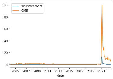
Google Trends

#!pip install pytrends
from pytrends.request import TrendReq
pytrend = TrendReq()
pytrend.build_payload(kw_list=['wallstreetbets','GME'],timeframe='all')
Googletrends=pytrend.interest_over_time()
Googletrends.plot()

<AxesSubplot:xlabel='date'>

WallStreet

• allow you to get real time data on stocks, calls, and put options

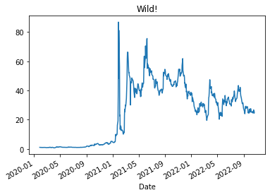
• Also allow you to very easily get historical data

• here is the manual:https://github.com/mcdallas/wallstreet

#!pip install wallstreet
from wallstreet import Stock, Call, Put
s = Stock('GME')

# this is the latest price of GME stock
s.price

25.3

# this gives you historical information
df = s.historical(days_back=1000, frequency='d')
df

	Date	Open	High	Low	Close	Adj Close	Volume
0	2020-01-27	1.050000	1.087500	1.040000	1.070000	1.070000	8490000
1	2020-01-28	1.075000	1.075000	1.045000	1.052500	1.052500	8579600
2	2020-01-29	1.055000	1.080000	1.032500	1.032500	1.032500	6210400
3	2020-01-30	1.025000	1.030000	0.970000	0.982500	0.982500	12026000
4	2020-01-31	0.977500	0.985000	0.957500	0.960000	0.960000	11566800
...	...	...	...	...	...	...	...
687	2022-10-17	25.370001	26.410000	25.240000	25.959999	25.959999	3172200
688	2022-10-18	27.100000	27.740000	26.129999	26.670000	26.670000	4402600
689	2022-10-19	26.000000	26.180000	24.270000	24.540001	24.540001	5318400
690	2022-10-20	24.650000	25.450001	24.070000	24.410000	24.410000	5148600
691	2022-10-21	24.150000	25.330000	24.100000	25.299999	25.299999	2999649

692 rows × 7 columns

df.set_index('Date').Close.plot()
plt.title('Wild!')

Text(0.5, 1.0, 'Wild!')

Pandas Datareader

this gives you acess to several data servers

For example the one that we used in Chapter 5.4

We will be particularly interested in the one Ken French updates with several quant strategies

Please check out https://pandas-datareader.readthedocs.io/en/latest/remote_data.html all the possiblities

#!pip install pandas_datareader
from pandas_datareader.famafrench import get_available_datasets
len(get_available_datasets())

297

There are 297 different data sets in Ken French library!

Below I show the full list. You can simply chose one to import, below I am import the '49_Industry_Portfolios' which has the portfolio of US stocks split in 49 industries.

In fact if you print the 'DESCR' field which contains the data set description you see that there are in fact 7 data sets as described below

from datetime import datetime
import pandas_datareader.data as web

start = datetime(1926, 1, 1) # this tell which month to start
ds = web.DataReader('49_Industry_Portfolios', 'famafrench',start=start)
print(ds['DESCR'])

49 Industry Portfolios
----------------------

This file was created by CMPT_IND_RETS using the 202103 CRSP database. It contains value- and equal-weighted returns for 49 industry portfolios. The portfolios are constructed at the end of June. The annual returns are from January to December. Missing data are indicated by -99.99 or -999. Copyright 2021 Kenneth R. French

  0 : Average Value Weighted Returns -- Monthly (1137 rows x 49 cols)
  1 : Average Equal Weighted Returns -- Monthly (1137 rows x 49 cols)
  2 : Average Value Weighted Returns -- Annual (94 rows x 49 cols)
  3 : Average Equal Weighted Returns -- Annual (94 rows x 49 cols)
  4 : Number of Firms in Portfolios (1137 rows x 49 cols)
  5 : Average Firm Size (1137 rows x 49 cols)
  6 : Sum of BE / Sum of ME (95 rows x 49 cols)
  7 : Value-Weighted Average of BE/ME (95 rows x 49 cols)

If you want Value weighted monthly returns you simply select 0

ds[0].tail()

	Agric	Food	Soda	Beer	Smoke	Toys	Fun	Books	Hshld	Clths	...	Boxes	Trans	Whlsl	Rtail	Meals	Banks	Insur	RlEst	Fin	Other
Date
2020-11	15.18	7.32	9.22	10.88	8.05	21.89	11.40	22.89	5.80	14.27	...	10.79	17.10	15.33	7.57	11.30	18.25	11.92	21.45	16.78	15.65
2020-12	1.33	1.90	6.84	3.33	8.67	15.77	9.79	10.83	0.86	4.63	...	2.46	0.73	3.04	1.08	4.05	7.55	4.42	9.68	8.24	1.78
2021-01	2.49	-1.32	-9.60	-6.89	-2.28	6.21	-3.77	3.66	-5.78	-4.84	...	-5.13	-4.58	-1.53	0.80	-4.52	-3.40	-3.85	3.87	-1.25	-1.76
2021-02	12.40	-0.04	0.66	-3.21	5.73	-2.33	10.42	13.70	-0.12	4.07	...	0.87	8.78	5.70	-3.17	7.97	14.29	4.11	18.83	9.31	5.98
2021-03	3.35	8.07	7.15	8.45	11.71	-8.30	-3.22	5.14	7.31	0.27	...	6.00	7.84	8.73	5.36	3.15	4.90	9.18	-1.24	4.11	6.03

5 rows × 49 columns

If you want the book to market ratio for each industry you select 6

ds[6].tail()

	Agric	Food	Soda	Beer	Smoke	Toys	Fun	Books	Hshld	Clths	...	Boxes	Trans	Whlsl	Rtail	Meals	Banks	Insur	RlEst	Fin	Other
Date
2016	0.16	0.35	0.13	0.12	0.10	0.28	0.22	0.80	0.23	0.20	...	0.36	0.32	0.31	0.22	0.12	0.83	0.72	0.40	0.66	0.36
2017	0.12	0.37	0.12	0.13	0.09	0.25	0.17	0.71	0.22	0.21	...	0.29	0.25	0.31	0.21	0.16	0.63	0.60	0.33	0.49	0.34
2018	0.46	0.46	0.10	0.14	0.14	0.21	0.13	0.61	0.24	0.16	...	0.37	0.29	0.32	0.16	0.14	0.57	0.58	0.30	0.46	0.40
2019	0.61	0.44	0.08	0.14	0.17	0.17	0.14	0.71	0.18	0.16	...	0.36	0.28	0.33	0.16	0.11	0.58	0.55	0.42	0.53	0.34
2020	1.14	0.45	0.10	0.17	0.09	0.20	0.14	0.80	0.15	0.16	...	0.40	0.31	0.33	0.14	0.23	0.75	0.69	0.56	0.55	0.49

5 rows × 49 columns

Below is the full list of datasets

get_available_datasets()

['F-F_Research_Data_Factors',
 'F-F_Research_Data_Factors_weekly',
 'F-F_Research_Data_Factors_daily',
 'F-F_Research_Data_5_Factors_2x3',
 'F-F_Research_Data_5_Factors_2x3_daily',
 'Portfolios_Formed_on_ME',
 'Portfolios_Formed_on_ME_Wout_Div',
 'Portfolios_Formed_on_ME_Daily',
 'Portfolios_Formed_on_BE-ME',
 'Portfolios_Formed_on_BE-ME_Wout_Div',
 'Portfolios_Formed_on_BE-ME_Daily',
 'Portfolios_Formed_on_OP',
 'Portfolios_Formed_on_OP_Wout_Div',
 'Portfolios_Formed_on_OP_Daily',
 'Portfolios_Formed_on_INV',
 'Portfolios_Formed_on_INV_Wout_Div',
 'Portfolios_Formed_on_INV_Daily',
 '6_Portfolios_2x3',
 '6_Portfolios_2x3_Wout_Div',
 '6_Portfolios_2x3_weekly',
 '6_Portfolios_2x3_daily',
 '25_Portfolios_5x5',
 '25_Portfolios_5x5_Wout_Div',
 '25_Portfolios_5x5_Daily',
 '100_Portfolios_10x10',
 '100_Portfolios_10x10_Wout_Div',
 '100_Portfolios_10x10_Daily',
 '6_Portfolios_ME_OP_2x3',
 '6_Portfolios_ME_OP_2x3_Wout_Div',
 '6_Portfolios_ME_OP_2x3_daily',
 '25_Portfolios_ME_OP_5x5',
 '25_Portfolios_ME_OP_5x5_Wout_Div',
 '25_Portfolios_ME_OP_5x5_daily',
 '100_Portfolios_ME_OP_10x10',
 '100_Portfolios_10x10_ME_OP_Wout_Div',
 '100_Portfolios_ME_OP_10x10_daily',
 '6_Portfolios_ME_INV_2x3',
 '6_Portfolios_ME_INV_2x3_Wout_Div',
 '6_Portfolios_ME_INV_2x3_daily',
 '25_Portfolios_ME_INV_5x5',
 '25_Portfolios_ME_INV_5x5_Wout_Div',
 '25_Portfolios_ME_INV_5x5_daily',
 '100_Portfolios_ME_INV_10x10',
 '100_Portfolios_10x10_ME_INV_Wout_Div',
 '100_Portfolios_ME_INV_10x10_daily',
 '25_Portfolios_BEME_OP_5x5',
 '25_Portfolios_BEME_OP_5x5_Wout_Div',
 '25_Portfolios_BEME_OP_5x5_daily',
 '25_Portfolios_BEME_INV_5x5',
 '25_Portfolios_BEME_INV_5x5_Wout_Div',
 '25_Portfolios_BEME_INV_5x5_daily',
 '25_Portfolios_OP_INV_5x5',
 '25_Portfolios_OP_INV_5x5_Wout_Div',
 '25_Portfolios_OP_INV_5x5_daily',
 '32_Portfolios_ME_BEME_OP_2x4x4',
 '32_Portfolios_ME_BEME_OP_2x4x4_Wout_Div',
 '32_Portfolios_ME_BEME_INV_2x4x4',
 '32_Portfolios_ME_BEME_INV_2x4x4_Wout_Div',
 '32_Portfolios_ME_OP_INV_2x4x4',
 '32_Portfolios_ME_OP_INV_2x4x4_Wout_Div',
 'Portfolios_Formed_on_E-P',
 'Portfolios_Formed_on_E-P_Wout_Div',
 'Portfolios_Formed_on_CF-P',
 'Portfolios_Formed_on_CF-P_Wout_Div',
 'Portfolios_Formed_on_D-P',
 'Portfolios_Formed_on_D-P_Wout_Div',
 '6_Portfolios_ME_EP_2x3',
 '6_Portfolios_ME_EP_2x3_Wout_Div',
 '6_Portfolios_ME_CFP_2x3',
 '6_Portfolios_ME_CFP_2x3_Wout_Div',
 '6_Portfolios_ME_DP_2x3',
 '6_Portfolios_ME_DP_2x3_Wout_Div',
 'F-F_Momentum_Factor',
 'F-F_Momentum_Factor_daily',
 '6_Portfolios_ME_Prior_12_2',
 '6_Portfolios_ME_Prior_12_2_Daily',
 '25_Portfolios_ME_Prior_12_2',
 '25_Portfolios_ME_Prior_12_2_Daily',
 '10_Portfolios_Prior_12_2',
 '10_Portfolios_Prior_12_2_Daily',
 'F-F_ST_Reversal_Factor',
 'F-F_ST_Reversal_Factor_daily',
 '6_Portfolios_ME_Prior_1_0',
 '6_Portfolios_ME_Prior_1_0_Daily',
 '25_Portfolios_ME_Prior_1_0',
 '25_Portfolios_ME_Prior_1_0_Daily',
 '10_Portfolios_Prior_1_0',
 '10_Portfolios_Prior_1_0_Daily',
 'F-F_LT_Reversal_Factor',
 'F-F_LT_Reversal_Factor_daily',
 '6_Portfolios_ME_Prior_60_13',
 '6_Portfolios_ME_Prior_60_13_Daily',
 '25_Portfolios_ME_Prior_60_13',
 '25_Portfolios_ME_Prior_60_13_Daily',
 '10_Portfolios_Prior_60_13',
 '10_Portfolios_Prior_60_13_Daily',
 'Portfolios_Formed_on_AC',
 '25_Portfolios_ME_AC_5x5',
 'Portfolios_Formed_on_BETA',
 '25_Portfolios_ME_BETA_5x5',
 'Portfolios_Formed_on_NI',
 '25_Portfolios_ME_NI_5x5',
 'Portfolios_Formed_on_VAR',
 '25_Portfolios_ME_VAR_5x5',
 'Portfolios_Formed_on_RESVAR',
 '25_Portfolios_ME_RESVAR_5x5',
 '5_Industry_Portfolios',
 '5_Industry_Portfolios_Wout_Div',
 '5_Industry_Portfolios_daily',
 '10_Industry_Portfolios',
 '10_Industry_Portfolios_Wout_Div',
 '10_Industry_Portfolios_daily',
 '12_Industry_Portfolios',
 '12_Industry_Portfolios_Wout_Div',
 '12_Industry_Portfolios_daily',
 '17_Industry_Portfolios',
 '17_Industry_Portfolios_Wout_Div',
 '17_Industry_Portfolios_daily',
 '30_Industry_Portfolios',
 '30_Industry_Portfolios_Wout_Div',
 '30_Industry_Portfolios_daily',
 '38_Industry_Portfolios',
 '38_Industry_Portfolios_Wout_Div',
 '38_Industry_Portfolios_daily',
 '48_Industry_Portfolios',
 '48_Industry_Portfolios_Wout_Div',
 '48_Industry_Portfolios_daily',
 '49_Industry_Portfolios',
 '49_Industry_Portfolios_Wout_Div',
 '49_Industry_Portfolios_daily',
 'ME_Breakpoints',
 'BE-ME_Breakpoints',
 'OP_Breakpoints',
 'INV_Breakpoints',
 'E-P_Breakpoints',
 'CF-P_Breakpoints',
 'D-P_Breakpoints',
 'Prior_2-12_Breakpoints',
 'Developed_3_Factors',
 'Developed_3_Factors_Daily',
 'Developed_ex_US_3_Factors',
 'Developed_ex_US_3_Factors_Daily',
 'Europe_3_Factors',
 'Europe_3_Factors_Daily',
 'Japan_3_Factors',
 'Japan_3_Factors_Daily',
 'Asia_Pacific_ex_Japan_3_Factors',
 'Asia_Pacific_ex_Japan_3_Factors_Daily',
 'North_America_3_Factors',
 'North_America_3_Factors_Daily',
 'Developed_5_Factors',
 'Developed_5_Factors_Daily',
 'Developed_ex_US_5_Factors',
 'Developed_ex_US_5_Factors_Daily',
 'Europe_5_Factors',
 'Europe_5_Factors_Daily',
 'Japan_5_Factors',
 'Japan_5_Factors_Daily',
 'Asia_Pacific_ex_Japan_5_Factors',
 'Asia_Pacific_ex_Japan_5_Factors_Daily',
 'North_America_5_Factors',
 'North_America_5_Factors_Daily',
 'Developed_Mom_Factor',
 'Developed_Mom_Factor_Daily',
 'Developed_ex_US_Mom_Factor',
 'Developed_ex_US_Mom_Factor_Daily',
 'Europe_Mom_Factor',
 'Europe_Mom_Factor_Daily',
 'Japan_Mom_Factor',
 'Japan_Mom_Factor_Daily',
 'Asia_Pacific_ex_Japan_MOM_Factor',
 'Asia_Pacific_ex_Japan_MOM_Factor_Daily',
 'North_America_Mom_Factor',
 'North_America_Mom_Factor_Daily',
 'Developed_6_Portfolios_ME_BE-ME',
 'Developed_6_Portfolios_ME_BE-ME_daily',
 'Developed_ex_US_6_Portfolios_ME_BE-ME',
 'Developed_ex_US_6_Portfolios_ME_BE-ME_daily',
 'Europe_6_Portfolios_ME_BE-ME',
 'Europe_6_Portfolios_ME_BE-ME_daily',
 'Japan_6_Portfolios_ME_BE-ME',
 'Japan_6_Portfolios_ME_BE-ME_daily',
 'Asia_Pacific_ex_Japan_6_Portfolios_ME_BE-ME',
 'Asia_Pacific_ex_Japan_6_Portfolios_ME_BE-ME_daily',
 'North_America_6_Portfolios_ME_BE-ME',
 'North_America_6_Portfolios_ME_BE-ME_daily',
 'Developed_25_Portfolios_ME_BE-ME',
 'Developed_25_Portfolios_ME_BE-ME_daily',
 'Developed_ex_US_25_Portfolios_ME_BE-ME',
 'Developed_ex_US_25_Portfolios_ME_BE-ME_daily',
 'Europe_25_Portfolios_ME_BE-ME',
 'Europe_25_Portfolios_ME_BE-ME_daily',
 'Japan_25_Portfolios_ME_BE-ME',
 'Japan_25_Portfolios_ME_BE-ME_daily',
 'Asia_Pacific_ex_Japan_25_Portfolios_ME_BE-ME',
 'Asia_Pacific_ex_Japan_25_Portfolios_ME_BE-ME_daily',
 'North_America_25_Portfolios_ME_BE-ME',
 'North_America_25_Portfolios_ME_BE-ME_daily',
 'Developed_6_Portfolios_ME_OP',
 'Developed_6_Portfolios_ME_OP_Daily',
 'Developed_ex_US_6_Portfolios_ME_OP',
 'Developed_ex_US_6_Portfolios_ME_OP_Daily',
 'Europe_6_Portfolios_ME_OP',
 'Europe_6_Portfolios_ME_OP_Daily',
 'Japan_6_Portfolios_ME_OP',
 'Japan_6_Portfolios_ME_OP_Daily',
 'Asia_Pacific_ex_Japan_6_Portfolios_ME_OP',
 'Asia_Pacific_ex_Japan_6_Portfolios_ME_OP_Daily',
 'North_America_6_Portfolios_ME_OP',
 'North_America_6_Portfolios_ME_OP_Daily',
 'Developed_25_Portfolios_ME_OP',
 'Developed_25_Portfolios_ME_OP_Daily',
 'Developed_ex_US_25_Portfolios_ME_OP',
 'Developed_ex_US_25_Portfolios_ME_OP_Daily',
 'Europe_25_Portfolios_ME_OP',
 'Europe_25_Portfolios_ME_OP_Daily',
 'Japan_25_Portfolios_ME_OP',
 'Japan_25_Portfolios_ME_OP_Daily',
 'Asia_Pacific_ex_Japan_25_Portfolios_ME_OP',
 'Asia_Pacific_ex_Japan_25_Portfolios_ME_OP_Daily',
 'North_America_25_Portfolios_ME_OP',
 'North_America_25_Portfolios_ME_OP_Daily',
 'Developed_6_Portfolios_ME_INV',
 'Developed_6_Portfolios_ME_INV_Daily',
 'Developed_ex_US_6_Portfolios_ME_INV',
 'Developed_ex_US_6_Portfolios_ME_INV_Daily',
 'Europe_6_Portfolios_ME_INV',
 'Europe_6_Portfolios_ME_INV_Daily',
 'Japan_6_Portfolios_ME_INV',
 'Japan_6_Portfolios_ME_INV_Daily',
 'Asia_Pacific_ex_Japan_6_Portfolios_ME_INV',
 'Asia_Pacific_ex_Japan_6_Portfolios_ME_INV_Daily',
 'North_America_6_Portfolios_ME_INV',
 'North_America_6_Portfolios_ME_INV_Daily',
 'Developed_25_Portfolios_ME_INV',
 'Developed_25_Portfolios_ME_INV_Daily',
 'Developed_ex_US_25_Portfolios_ME_INV',
 'Developed_ex_US_25_Portfolios_ME_INV_Daily',
 'Europe_25_Portfolios_ME_INV',
 'Europe_25_Portfolios_ME_INV_Daily',
 'Japan_25_Portfolios_ME_INV',
 'Japan_25_Portfolios_ME_INV_Daily',
 'Asia_Pacific_ex_Japan_25_Portfolios_ME_INV',
 'Asia_Pacific_ex_Japan_25_Portfolios_ME_INV_Daily',
 'North_America_25_Portfolios_ME_INV',
 'North_America_25_Portfolios_ME_INV_Daily',
 'Developed_6_Portfolios_ME_Prior_12_2',
 'Developed_6_Portfolios_ME_Prior_250_20_daily',
 'Developed_ex_US_6_Portfolios_ME_Prior_12_2',
 'Developed_ex_US_6_Portfolios_ME_Prior_250_20_daily',
 'Europe_6_Portfolios_ME_Prior_12_2',
 'Europe_6_Portfolios_ME_Prior_250_20_daily',
 'Japan_6_Portfolios_ME_Prior_12_2',
 'Japan_6_Portfolios_ME_Prior_250_20_daily',
 'Asia_Pacific_ex_Japan_6_Portfolios_ME_Prior_12_2',
 'Asia_Pacific_ex_Japan_6_Portfolios_ME_Prior_250_20_daily',
 'North_America_6_Portfolios_ME_Prior_12_2',
 'North_America_6_Portfolios_ME_Prior_250_20_daily',
 'Developed_25_Portfolios_ME_Prior_12_2',
 'Developed_25_Portfolios_ME_Prior_250_20_daily',
 'Developed_ex_US_25_Portfolios_ME_Prior_12_2',
 'Developed_ex_US_25_Portfolios_ME_Prior_250_20_daily',
 'Europe_25_Portfolios_ME_Prior_12_2',
 'Europe_25_Portfolios_ME_Prior_250_20_daily',
 'Japan_25_Portfolios_ME_Prior_12_2',
 'Japan_25_Portfolios_ME_Prior_250_20_daily',
 'Asia_Pacific_ex_Japan_25_Portfolios_ME_Prior_12_2',
 'Asia_Pacific_ex_Japan_25_Portfolios_ME_Prior_250_20_daily',
 'North_America_25_Portfolios_ME_Prior_12_2',
 'North_America_25_Portfolios_ME_Prior_250_20_daily',
 'Developed_32_Portfolios_ME_BE-ME_OP_2x4x4',
 'Developed_ex_US_32_Portfolios_ME_BE-ME_OP_2x4x4',
 'Europe_32_Portfolios_ME_BE-ME_OP_2x4x4',
 'Japan_32_Portfolios_ME_BE-ME_OP_2x4x4',
 'Asia_Pacific_ex_Japan_32_Portfolios_ME_BE-ME_OP_2x4x4',
 'North_America_32_Portfolios_ME_BE-ME_OP_2x4x4',
 'Developed_32_Portfolios_ME_BE-ME_INV(TA)_2x4x4',
 'Developed_ex_US_32_Portfolios_ME_BE-ME_INV(TA)_2x4x4',
 'Europe_32_Portfolios_ME_BE-ME_INV(TA)_2x4x4',
 'Japan_32_Portfolios_ME_BE-ME_INV(TA)_2x4x4',
 'Asia_Pacific_ex_Japan_32_Portfolios_ME_BE-ME_INV(TA)_2x4x4',
 'North_America_32_Portfolios_ME_BE-ME_INV(TA)_2x4x4',
 'Developed_32_Portfolios_ME_INV(TA)_OP_2x4x4',
 'Developed_ex_US_32_Portfolios_ME_INV(TA)_OP_2x4x4',
 'Europe_32_Portfolios_ME_INV(TA)_OP_2x4x4',
 'Japan_32_Portfolios_ME_INV(TA)_OP_2x4x4',
 'Asia_Pacific_ex_Japan_32_Portfolios_ME_INV(TA)_OP_2x4x4',
 'North_America_32_Portfolios_ME_INV(TA)_OP_2x4x4',
 'Emerging_5_Factors',
 'Emerging_MOM_Factor',
 'Emerging_Markets_6_Portfolios_ME_BE-ME',
 'Emerging_Markets_6_Portfolios_ME_OP',
 'Emerging_Markets_6_Portfolios_ME_INV',
 'Emerging_Markets_6_Portfolios_ME_Prior_12_2',
 'Emerging_Markets_4_Portfolios_BE-ME_OP',
 'Emerging_Markets_4_Portfolios_OP_INV',
 'Emerging_Markets_4_Portfolios_BE-ME_INV']

WRDS

This is harder and more sophisticated

You DONT NEED TO USE THIS IF YOU DONT WANT!

WRDS has all sorts of amazing data for finance. For equity prices and mutual funds in particular.

You can easily register for an account here https://wrds-www.wharton.upenn.edu/register/

In this class we will use it go get stock market data and also data on company earnigns and other balance sheet information

Google/Yahoo finance data are nice to play with, but they tend to have errors in it. So if you are doing serious work I will probably advise agaist using them only.

WRDS is really the gold standard, but the data publication lag is long, so you can use it to do research, but not to trade

To use it you have to load two libraries

#!pip install wrds
import wrds
import psycopg2 

Collecting wrds
  Downloading wrds-3.1.2-py3-none-any.whl (13 kB)
Requirement already satisfied: sqlalchemy in c:\users\alan.moreira\anaconda3\lib\site-packages (from wrds) (1.4.32)
Collecting psycopg2-binary
  Downloading psycopg2_binary-2.9.4-cp39-cp39-win_amd64.whl (1.2 MB)
Requirement already satisfied: mock in c:\users\alan.moreira\anaconda3\lib\site-packages (from wrds) (4.0.3)
Requirement already satisfied: pandas in c:\users\alan.moreira\anaconda3\lib\site-packages (from wrds) (1.4.2)
Requirement already satisfied: numpy in c:\users\alan.moreira\anaconda3\lib\site-packages (from wrds) (1.21.5)
Requirement already satisfied: pytz>=2020.1 in c:\users\alan.moreira\anaconda3\lib\site-packages (from pandas->wrds) (2021.3)
Requirement already satisfied: python-dateutil>=2.8.1 in c:\users\alan.moreira\anaconda3\lib\site-packages (from pandas->wrds) (2.8.2)
Requirement already satisfied: six>=1.5 in c:\users\alan.moreira\anaconda3\lib\site-packages (from python-dateutil>=2.8.1->pandas->wrds) (1.16.0)
Requirement already satisfied: greenlet!=0.4.17 in c:\users\alan.moreira\anaconda3\lib\site-packages (from sqlalchemy->wrds) (1.1.1)
Installing collected packages: psycopg2-binary, wrds
Successfully installed psycopg2-binary-2.9.4 wrds-3.1.2

You then initiate a connection when you are requested to type your pasword and username

conn=wrds.Connection()

Enter your WRDS username [Alan.Moreira]: moreira5
Enter your password: ···········

WRDS recommends setting up a .pgpass file.

Create .pgpass file now [y/n]?:  y

Created .pgpass file successfully.
Loading library list...
Done

With this connection you can use their SQL interface to get the desired data

Here I recommend most copying and pasting code across the web.

This website by Freda Drechsler provides lots of guidance and code on how to do it

https://www.fredasongdrechsler.com/intro-to-python-for-fnce/maneuvering-wrds-data

and also has lots of code that teaches you how to get both financial and accouting information from WRDS, for example, (https://www.fredasongdrechsler.com/full-python-code/dgtw)

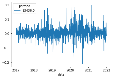
Below we will simply write a function that dowloads dailt return data for a given firm

def get_returns(tickers,conn,startdate,enddate):
    ticker=tickers[0]
    df = conn.raw_sql("""
                          select a.permno, b.ticker, a.date,a.ret 
                          from crsp.dsf as a
                          left join crsp.msenames as b
                          on a.permno=b.permno
                          and b.namedt<=a.date
                          and a.date<=b.nameendt
                          where a.date between '"""+ startdate+"""'  and '"""+ enddate+            
                          """' and  b.ticker='"""+ticker+"'")
            
    df.set_index(['date','permno'],inplace=True)
    df=df['ret'].unstack()
    return df

df=get_returns(['TSLA'],conn,'1/1/2017','1/1/2022')
df.plot()

<AxesSubplot:xlabel='date'>

If I wanted other information I would have to know this information is named in the database

For example,

• vol gets tradign volume (in shares),

• prc gets the unadjusted price,

• retx gets returns without dividends

• shrout gets share outstanding

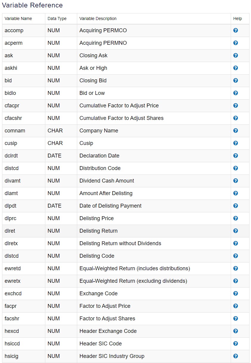
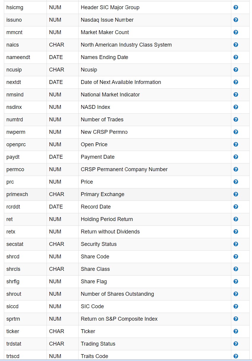
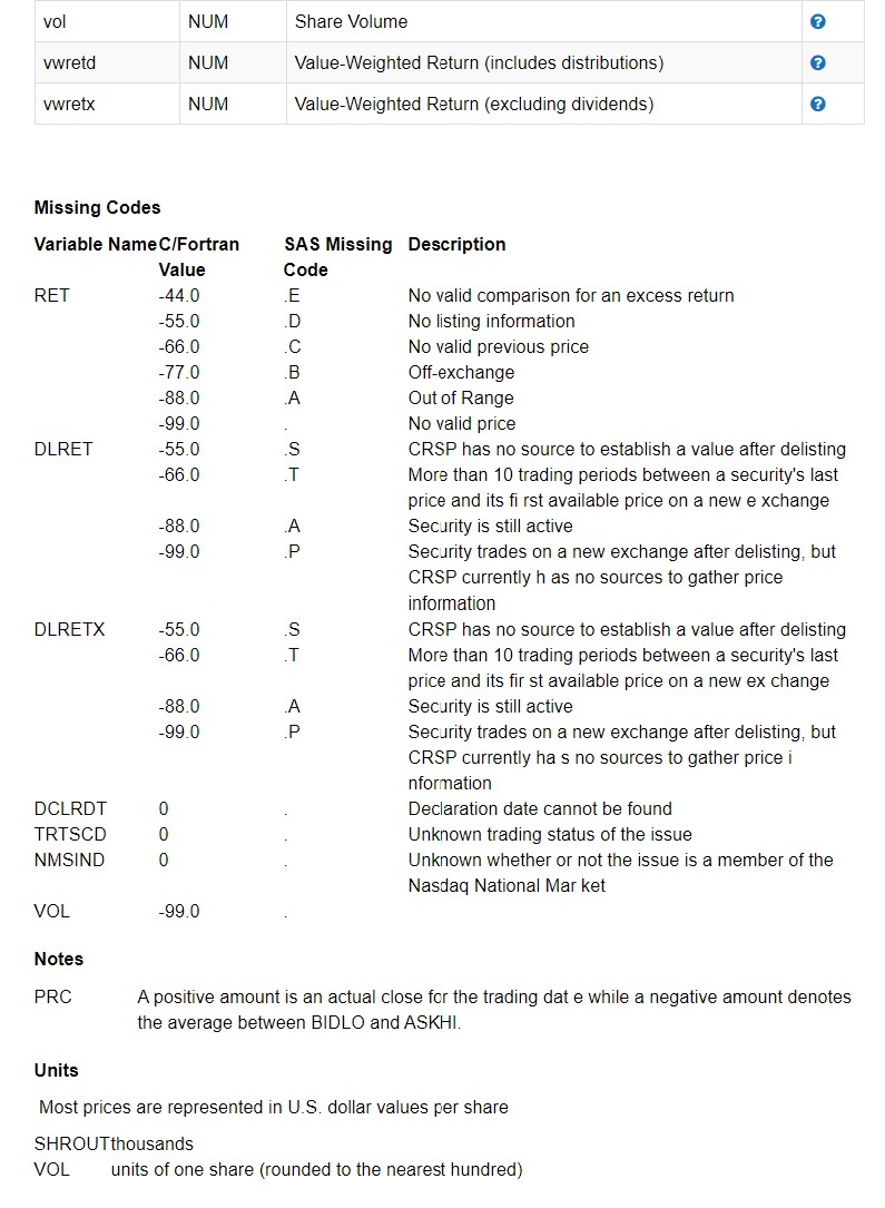
In the end of this notebook you put a list of data that this particular data set in wrds allow you easy access to.It also has a description of how missing values are handled.

To construct the market cap you need both the price and the shareoutstanding, which you can easily download with a single function call by adding to your code

def get_data(tickers,conn,startdate,enddate):
    ticker=tickers[0]
    df = conn.raw_sql("""
                          select a.permno, b.ticker, a.date,a.prc,a.shrout 
                          from crsp.dsf as a
                          left join crsp.msenames as b
                          on a.permno=b.permno
                          and b.namedt<=a.date
                          and a.date<=b.nameendt
                          where a.date between '"""+ startdate+"""'  and '"""+ enddate+            
                          """' and  b.ticker='"""+ticker+"'")
            
    df.set_index(['date','permno'],inplace=True)
 #   I commented out this step because now I would like to get more than one variable so I cannot unstack
  #  df=df[variable].unstack()
    return df

df=get_data(['TSLA'],conn,'1/1/2005','1/1/2022')
df.tail()

		ticker	prc	shrout
date	permno
2021-12-27	93436.0	TSLA	1093.939941	1004265.0
2021-12-28	93436.0	TSLA	1088.469971	1004265.0
2021-12-29	93436.0	TSLA	1086.189941	1004265.0
2021-12-30	93436.0	TSLA	1070.339966	1004265.0
2021-12-31	93436.0	TSLA	1056.780029	1033534.0

df['mcap']=df.prc.abs()*df.shrout
# the use a negative price to say that the price is not based on end of day transaction 
#but a mid price between bid and ask
df.mcap.plot()

<AxesSubplot:xlabel='date,permno'>

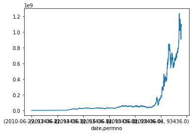
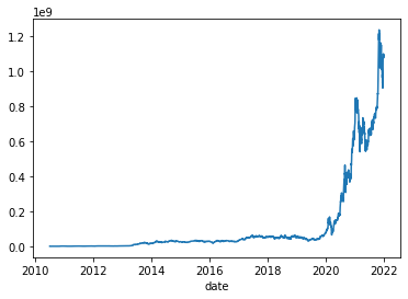
This is ugly because we have the permno, the indentity of security as an index. To fix this, lets take this out of the index

df=df.reset_index().set_index('date')
df.mcap.plot()

<AxesSubplot:xlabel='date'>

Variable reference for WRDS CRSP data set