
Time series
Contents
5.4. Time series#
import numpy as np
import pandas as pd
import matplotlib.pyplot as plt
5.4.1. Intro#
pandas has extensive support for handling dates and times.
We will loosely refer to data with date or time information as time series data.
In this lecture, we will cover the most useful parts of pandas’ time series functionality.
Among these topics are:
Parsing strings as dates
Writing
datetimeobjects as (inverse operation of previous point)Extracting data from a DataFrame or Series with date information in the index
Shifting data through time (taking leads or lags)
Re-sampling data to a different frequency and rolling operations
However, even more than with previous topics, we will skip a lot of the functionality pandas offers, and we urge you to refer to the official documentation for more information.
5.4.2. Parsing Strings as Dates#
When working with time series data, we almost always receive the data with dates encoded as strings.
Hopefully, the date strings follow a structured format or pattern.
One common pattern is YYYY-MM-DD: 4 numbers for the year, 2 for the
month, and 2 for the day with each section separated by a -.
For example, we write Christmas day 2017 in this format as
christmas_str = "2017-12-25"
To convert a string into a time-aware object, we use the
pd.to_datetime function.
christmas = pd.to_datetime(christmas_str)
print("The type of christmas is", type(christmas))
christmas
The type of christmas is <class 'pandas._libs.tslibs.timestamps.Timestamp'>
Timestamp('2017-12-25 00:00:00')
The pd.to_datetime function is pretty smart at guessing the format
of the date…
for date in ["December 25, 2017", "Dec. 25, 2017",
             "Monday, Dec. 25, 2017", "25 Dec. 2017", "25th Dec. 2017"]:
    print("pandas interprets {} as {}".format(date, pd.to_datetime(date)))
pandas interprets December 25, 2017 as 2017-12-25 00:00:00
pandas interprets Dec. 25, 2017 as 2017-12-25 00:00:00
pandas interprets Monday, Dec. 25, 2017 as 2017-12-25 00:00:00
pandas interprets 25 Dec. 2017 as 2017-12-25 00:00:00
pandas interprets 25th Dec. 2017 as 2017-12-25 00:00:00
However, sometimes we will need to give pandas a hint.
For example, that same time (midnight on Christmas) would be reported on an Amazon transaction report as
christmas_amzn = "2017-12-25T00:00:00+ 00 :00"
If we try to pass this to pd.to_datetime, it will fail.
pd.to_datetime(christmas_amzn)
To parse a date with this format, we need to specify the format
argument for pd.to_datetime.
amzn_strftime = "%Y-%m-%dT%H:%M:%S+ 00 :00"
pd.to_datetime(christmas_amzn, format=amzn_strftime)
Timestamp('2017-12-25 00:00:00')
Can you guess what amzn_strftime represents?
Let’s take a closer look at amzn_strftime and christmas_amzn.
print(amzn_strftime)
print(christmas_amzn)
%Y-%m-%dT%H:%M:%S+ 00 :00
2017-12-25T00:00:00+ 00 :00
Notice that both of the strings have a similar form, but that instead of actual numerical values, amzn_strftime has placeholders.
Specifically, anywhere the % shows up is a signal to the pd.to_datetime
function that it is where relevant information is stored.
For example, the %Y is a stand-in for a four digit year, %m is
for 2 a digit month, and so on…
The official Python
documentation contains a complete list of possible %something patterns that are accepted
in the format argument.
5.4.2.1. Multiple Dates#
If we have dates in a Series (e.g. column of DataFrame) or a list, we
can pass the entire collection to pd.to_datetime and get a
collection of dates back.
We’ll just show an example of that here as the mechanics are the same as a single date.
pd.to_datetime(["2017-12-25", "2017-12-31"])
DatetimeIndex(['2017-12-25', '2017-12-31'], dtype='datetime64[ns]', freq=None)
5.4.3. Extracting Data#
When the index of a DataFrame has date information and pandas
recognizes the values as datetime values, we can leverage some
convenient indexing features for extracting data.
The flexibility of these features is best understood through example, so let’s load up some data and take a look.
Below we are using pandas data reader API that allows us to get Alpha Advantadge finance data for free look here
You can apply for a free API key here https://www.alphavantage.co/support/#api-key
There is a wide range of different API for Python. We will later discuss a few more that we will use
import pandas_datareader.data as pdr
import datetime as dt

# yahoo, not currently working
#df = web.DataReader('GME', 'yahoo', start='2019-09-10', end='2019-10-09')

# alpha vantage, require api key
gme= pdr.DataReader("GME", "av-daily", start=dt.datetime(2013, 1, 2),
                      end=dt.datetime(2021, 11, 1),
                     api_key='N78MZQUK4ZCDUABU')


gme.tail()
| open | high | low | close | volume | |
|---|---|---|---|---|---|
| 2021-10-26 | 173.36 | 185.00 | 172.50 | 177.84 | 2176749 |
| 2021-10-27 | 180.00 | 183.09 | 172.33 | 173.51 | 1106998 |
| 2021-10-28 | 175.16 | 183.14 | 175.00 | 182.85 | 1696206 |
| 2021-10-29 | 182.81 | 185.75 | 178.00 | 183.51 | 2293970 |
| 2021-11-01 | 182.53 | 208.57 | 182.05 | 200.09 | 4910802 |
LEts start by getting prices back in 2015
#gme.loc["2015"]
What did go wrong?
gme.info()
<class 'pandas.core.frame.DataFrame'>
Index: 2225 entries, 2013-01-02 to 2021-11-01
Data columns (total 5 columns):
 #   Column  Non-Null Count  Dtype
---  ------  --------------  -----
 0   open    2225 non-null   float64
 1   high    2225 non-null   float64
 2   low     2225 non-null   float64
 3   close   2225 non-null   float64
 4   volume  2225 non-null   int64
dtypes: float64(4), int64(1)
memory usage: 104.3+ KB
Lets make sure that the index is interpeted as Date
gme.index=pd.to_datetime(gme.index)
gme.info()
<class 'pandas.core.frame.DataFrame'>
DatetimeIndex: 2225 entries, 2013-01-02 to 2021-11-01
Data columns (total 5 columns):
 #   Column  Non-Null Count  Dtype
---  ------  --------------  -----
 0   open    2225 non-null   float64
 1   high    2225 non-null   float64
 2   low     2225 non-null   float64
 3   close   2225 non-null   float64
 4   volume  2225 non-null   int64
dtypes: float64(4), int64(1)
memory usage: 104.3 KB
Here, we have the Game Stop from 2013 until today.
Notice that the type of index is DateTimeIndex.
This is the key that enables things like…
Extracting all data for the year 2015 by passing "2015" to .loc.
gme.loc["2015"]
| open | high | low | close | volume | |
|---|---|---|---|---|---|
| 2015-01-02 | 34.06 | 34.1600 | 33.2500 | 33.80 | 1612946 |
| 2015-01-05 | 33.52 | 34.8800 | 33.3300 | 34.72 | 4940754 |
| 2015-01-06 | 35.17 | 36.0300 | 33.5200 | 33.69 | 4885107 |
| 2015-01-07 | 34.29 | 34.6800 | 32.9800 | 33.30 | 2558324 |
| 2015-01-08 | 33.60 | 34.1700 | 33.3200 | 33.69 | 4547436 |
| ... | ... | ... | ... | ... | ... |
| 2015-12-24 | 28.62 | 28.8000 | 28.2799 | 28.37 | 868965 |
| 2015-12-28 | 28.37 | 28.9400 | 28.1400 | 28.47 | 2325435 |
| 2015-12-29 | 28.62 | 28.8000 | 28.3268 | 28.43 | 2041056 |
| 2015-12-30 | 28.37 | 28.9399 | 28.2400 | 28.48 | 1438398 |
| 2015-12-31 | 28.43 | 28.8600 | 28.0300 | 28.04 | 1696030 |
252 rows × 5 columns
We can also narrow down to specific months.
# By month's name
gme.loc["August 2017"]
| open | high | low | close | volume | |
|---|---|---|---|---|---|
| 2017-08-01 | 21.69 | 21.690 | 21.1400 | 21.36 | 3059060 |
| 2017-08-02 | 21.32 | 21.620 | 21.2718 | 21.38 | 1114494 |
| 2017-08-03 | 21.32 | 21.820 | 21.3200 | 21.66 | 1047946 |
| 2017-08-04 | 21.78 | 22.110 | 21.6874 | 21.93 | 1136118 |
| 2017-08-07 | 21.94 | 22.255 | 21.8250 | 22.17 | 1276275 |
| 2017-08-08 | 22.20 | 22.370 | 21.9000 | 21.94 | 1422533 |
| 2017-08-09 | 21.75 | 22.120 | 21.6200 | 22.08 | 1502404 |
| 2017-08-10 | 21.91 | 21.910 | 21.4600 | 21.47 | 1517745 |
| 2017-08-11 | 21.24 | 21.830 | 21.0700 | 21.76 | 1616078 |
| 2017-08-14 | 21.95 | 21.990 | 21.7150 | 21.85 | 1532902 |
| 2017-08-15 | 21.70 | 21.770 | 20.7800 | 20.93 | 3886017 |
| 2017-08-16 | 21.12 | 21.490 | 21.0800 | 21.39 | 2412361 |
| 2017-08-17 | 21.37 | 21.660 | 21.0000 | 21.10 | 1928060 |
| 2017-08-18 | 21.05 | 21.330 | 20.9700 | 21.22 | 2117015 |
| 2017-08-21 | 21.16 | 21.360 | 20.9700 | 20.98 | 1633080 |
| 2017-08-22 | 21.12 | 21.690 | 21.0900 | 21.64 | 2468755 |
| 2017-08-23 | 21.59 | 21.820 | 21.2100 | 21.48 | 2428181 |
| 2017-08-24 | 21.75 | 22.120 | 21.6500 | 21.78 | 3669710 |
| 2017-08-25 | 19.90 | 19.940 | 18.7200 | 19.40 | 20500700 |
| 2017-08-28 | 19.41 | 19.700 | 18.9600 | 19.15 | 5213366 |
| 2017-08-29 | 18.93 | 19.070 | 18.6400 | 18.75 | 4663522 |
| 2017-08-30 | 18.75 | 18.970 | 18.6800 | 18.79 | 2209062 |
| 2017-08-31 | 18.83 | 18.870 | 18.4700 | 18.50 | 2625788 |
# By month's number
gme.loc["08/2017"]
| open | high | low | close | volume | |
|---|---|---|---|---|---|
| 2017-08-01 | 21.69 | 21.690 | 21.1400 | 21.36 | 3059060 |
| 2017-08-02 | 21.32 | 21.620 | 21.2718 | 21.38 | 1114494 |
| 2017-08-03 | 21.32 | 21.820 | 21.3200 | 21.66 | 1047946 |
| 2017-08-04 | 21.78 | 22.110 | 21.6874 | 21.93 | 1136118 |
| 2017-08-07 | 21.94 | 22.255 | 21.8250 | 22.17 | 1276275 |
| 2017-08-08 | 22.20 | 22.370 | 21.9000 | 21.94 | 1422533 |
| 2017-08-09 | 21.75 | 22.120 | 21.6200 | 22.08 | 1502404 |
| 2017-08-10 | 21.91 | 21.910 | 21.4600 | 21.47 | 1517745 |
| 2017-08-11 | 21.24 | 21.830 | 21.0700 | 21.76 | 1616078 |
| 2017-08-14 | 21.95 | 21.990 | 21.7150 | 21.85 | 1532902 |
| 2017-08-15 | 21.70 | 21.770 | 20.7800 | 20.93 | 3886017 |
| 2017-08-16 | 21.12 | 21.490 | 21.0800 | 21.39 | 2412361 |
| 2017-08-17 | 21.37 | 21.660 | 21.0000 | 21.10 | 1928060 |
| 2017-08-18 | 21.05 | 21.330 | 20.9700 | 21.22 | 2117015 |
| 2017-08-21 | 21.16 | 21.360 | 20.9700 | 20.98 | 1633080 |
| 2017-08-22 | 21.12 | 21.690 | 21.0900 | 21.64 | 2468755 |
| 2017-08-23 | 21.59 | 21.820 | 21.2100 | 21.48 | 2428181 |
| 2017-08-24 | 21.75 | 22.120 | 21.6500 | 21.78 | 3669710 |
| 2017-08-25 | 19.90 | 19.940 | 18.7200 | 19.40 | 20500700 |
| 2017-08-28 | 19.41 | 19.700 | 18.9600 | 19.15 | 5213366 |
| 2017-08-29 | 18.93 | 19.070 | 18.6400 | 18.75 | 4663522 |
| 2017-08-30 | 18.75 | 18.970 | 18.6800 | 18.79 | 2209062 |
| 2017-08-31 | 18.83 | 18.870 | 18.4700 | 18.50 | 2625788 |
Or even a day…
# By date name
gme.loc["August 1, 2017"]
open           21.69
high           21.69
low            21.14
close          21.36
volume    3059060.00
Name: 2017-08-01 00:00:00, dtype: float64
# By date number
gme.loc["08-01-2017"]
open           21.69
high           21.69
low            21.14
close          21.36
volume    3059060.00
Name: 2017-08-01 00:00:00, dtype: float64
What can we pass as the .loc argument when we have a
DateTimeIndex?
Anything that can be converted to a datetime using
pd.to_datetime, without having to specify the format argument.
When that condition holds, pandas will return all rows whose date in the index “belong” to that date or period.
We can also use the range shorthand notation to give a start and end date for selection.
gme.loc["April 1, 2015":"April 10, 2015"]
| open | high | low | close | volume | |
|---|---|---|---|---|---|
| 2015-04-01 | 37.86 | 38.50 | 37.330 | 37.78 | 2464874 |
| 2015-04-02 | 38.06 | 38.81 | 37.880 | 38.20 | 1172602 |
| 2015-04-06 | 38.00 | 38.39 | 37.680 | 38.37 | 1483853 |
| 2015-04-07 | 38.37 | 38.50 | 37.915 | 37.98 | 1332103 |
| 2015-04-08 | 37.80 | 38.78 | 37.740 | 38.71 | 1649946 |
| 2015-04-09 | 38.76 | 40.00 | 38.350 | 39.99 | 1912082 |
| 2015-04-10 | 40.18 | 40.41 | 39.560 | 40.40 | 1268980 |
5.4.4. Accessing Date Properties#
Sometimes, we would like to directly access a part of the date/time.
If our date/time information is in the index, we can to df.index.XX
where XX is replaced by year, month, or whatever we would
like to access.
gme.index.year
Int64Index([2013, 2013, 2013, 2013, 2013, 2013, 2013, 2013, 2013, 2013,
            ...
            2021, 2021, 2021, 2021, 2021, 2021, 2021, 2021, 2021, 2021],
           dtype='int64', length=2225)
gme.index.day
Int64Index([ 2,  3,  4,  7,  8,  9, 10, 11, 14, 15,
            ...
            19, 20, 21, 22, 25, 26, 27, 28, 29,  1],
           dtype='int64', length=2225)
We can also do the same if the date/time information is stored in a column, but we have to use a slightly different syntax.
df["column_name"].dt.XX
gme_date_column = gme.reset_index()
gme_date_column.head()
| index | open | high | low | close | volume | |
|---|---|---|---|---|---|---|
| 0 | 2013-01-02 | 25.58 | 25.870 | 24.99 | 25.66 | 4898100 |
| 1 | 2013-01-03 | 25.58 | 25.685 | 23.92 | 24.36 | 10642800 |
| 2 | 2013-01-04 | 24.42 | 25.170 | 24.36 | 24.80 | 4040000 |
| 3 | 2013-01-07 | 24.66 | 24.920 | 23.87 | 24.75 | 3983900 |
| 4 | 2013-01-08 | 22.93 | 23.960 | 22.66 | 23.19 | 11131200 |
gme_date_column["index"].dt.year.head()
0    2013
1    2013
2    2013
3    2013
4    2013
Name: index, dtype: int64
gme_date_column["index"].dt.month.head()
0    1
1    1
2    1
3    1
4    1
Name: index, dtype: int64
5.4.5. Leads and Lags: df.shift#
When doing time series analysis, we often want to compare data at one date against data at another date.
pandas can help us with this if we leverage the shift method.
Without any additional arguments, shift() will move all data
forward one period, filling the first row with missing data.
# so we can see the result of shift clearly
gme.head()
| open | high | low | close | volume | |
|---|---|---|---|---|---|
| 2013-01-02 | 25.58 | 25.870 | 24.99 | 25.66 | 4898100 |
| 2013-01-03 | 25.58 | 25.685 | 23.92 | 24.36 | 10642800 |
| 2013-01-04 | 24.42 | 25.170 | 24.36 | 24.80 | 4040000 |
| 2013-01-07 | 24.66 | 24.920 | 23.87 | 24.75 | 3983900 |
| 2013-01-08 | 22.93 | 23.960 | 22.66 | 23.19 | 11131200 |
gme.shift().head()
| open | high | low | close | volume | |
|---|---|---|---|---|---|
| 2013-01-02 | NaN | NaN | NaN | NaN | NaN |
| 2013-01-03 | 25.58 | 25.870 | 24.99 | 25.66 | 4898100.0 |
| 2013-01-04 | 25.58 | 25.685 | 23.92 | 24.36 | 10642800.0 |
| 2013-01-07 | 24.42 | 25.170 | 24.36 | 24.80 | 4040000.0 |
| 2013-01-08 | 24.66 | 24.920 | 23.87 | 24.75 | 3983900.0 |
We can use this to compute the percent change from one day to the next. (Quiz: Why does that work? Remember how pandas uses the index to align data.)
((gme.close - gme.close.shift()) / gme.close.shift()).head()
2013-01-02         NaN
2013-01-03   -0.050663
2013-01-04    0.018062
2013-01-07   -0.002016
2013-01-08   -0.063030
Name: close, dtype: float64
Setting the first argument to n tells pandas to shift the data down
n rows (apply an n period lag).
gme.shift(3).head()
| open | high | low | close | volume | |
|---|---|---|---|---|---|
| 2013-01-02 | NaN | NaN | NaN | NaN | NaN |
| 2013-01-03 | NaN | NaN | NaN | NaN | NaN |
| 2013-01-04 | NaN | NaN | NaN | NaN | NaN |
| 2013-01-07 | 25.58 | 25.870 | 24.99 | 25.66 | 4898100.0 |
| 2013-01-08 | 25.58 | 25.685 | 23.92 | 24.36 | 10642800.0 |
A negative value will shift the data up or apply a lead.
gme.shift(-2).tail()
| open | high | low | close | volume | |
|---|---|---|---|---|---|
| 2021-10-26 | 175.16 | 183.14 | 175.00 | 182.85 | 1696206.0 |
| 2021-10-27 | 182.81 | 185.75 | 178.00 | 183.51 | 2293970.0 |
| 2021-10-28 | 182.53 | 208.57 | 182.05 | 200.09 | 4910802.0 |
| 2021-10-29 | NaN | NaN | NaN | NaN | NaN |
| 2021-11-01 | NaN | NaN | NaN | NaN | NaN |
gme.shift(-2).head()
| open | high | low | close | volume | |
|---|---|---|---|---|---|
| 2013-01-02 | 24.42 | 25.17 | 24.36 | 24.80 | 4040000.0 |
| 2013-01-03 | 24.66 | 24.92 | 23.87 | 24.75 | 3983900.0 |
| 2013-01-04 | 22.93 | 23.96 | 22.66 | 23.19 | 11131200.0 |
| 2013-01-07 | 23.12 | 23.32 | 22.52 | 22.61 | 4331900.0 |
| 2013-01-08 | 22.81 | 22.88 | 22.40 | 22.79 | 3900300.0 |
5.4.6. Rolling Computations: .rolling#
pandas has facilities that enable easy computation of rolling statistics.
These are best understood by example, so we will dive right in.
# first take only the first 6 rows so we can easily see what is going on
gme_small = gme.head(6)
gme_small
| open | high | low | close | volume | |
|---|---|---|---|---|---|
| 2013-01-02 | 25.58 | 25.870 | 24.99 | 25.66 | 4898100 |
| 2013-01-03 | 25.58 | 25.685 | 23.92 | 24.36 | 10642800 |
| 2013-01-04 | 24.42 | 25.170 | 24.36 | 24.80 | 4040000 |
| 2013-01-07 | 24.66 | 24.920 | 23.87 | 24.75 | 3983900 |
| 2013-01-08 | 22.93 | 23.960 | 22.66 | 23.19 | 11131200 |
| 2013-01-09 | 23.12 | 23.320 | 22.52 | 22.61 | 4331900 |
Below, we compute the 2 day moving average (for all columns).
gme_small.rolling("2d").mean()
| open | high | low | close | volume | |
|---|---|---|---|---|---|
| 2013-01-02 | 25.580 | 25.8700 | 24.990 | 25.66 | 4898100.0 |
| 2013-01-03 | 25.580 | 25.7775 | 24.455 | 25.01 | 7770450.0 |
| 2013-01-04 | 25.000 | 25.4275 | 24.140 | 24.58 | 7341400.0 |
| 2013-01-07 | 24.660 | 24.9200 | 23.870 | 24.75 | 3983900.0 |
| 2013-01-08 | 23.795 | 24.4400 | 23.265 | 23.97 | 7557550.0 |
| 2013-01-09 | 23.025 | 23.6400 | 22.590 | 22.90 | 7731550.0 |
To do this operation, pandas starts at each row (date) then looks
backwards the specified number of periods (here 2 days) and then
applies some aggregation function (mean) on all the data in that
window.
If pandas cannot look back the full length of the window (e.g. when working on the first row), it fills as much of the window as possible and then does the operation. Notice that the value at 2013-02-25 is the same in both DataFrames.
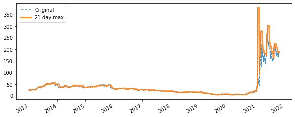
Below, we see a visual depiction of the rolling maximum on a 21 day window for the whole dataset.
fig, ax = plt.subplots(figsize=(10, 4))
gme["open"].plot(ax=ax, linestyle="--", alpha=0.8)
gme.rolling("21d").max()["open"].plot(ax=ax, alpha=0.8, linewidth=3)
ax.legend(["Original", "21 day max"])
<matplotlib.legend.Legend at 0x1c4d19cd3a0>
We can also ask pandas to apply custom functions, similar to what we
saw when studying GroupBy.
def is_volatile(x):
    "Returns a 1 if the variance is greater than 1, otherwise returns 0"
    if x.var() > 1.0:
        return 1.0
    else:
        return 0.0
gme_small.open.rolling("21d").apply(is_volatile)
2013-01-02    0.0
2013-01-03    0.0
2013-01-04    0.0
2013-01-07    0.0
2013-01-08    1.0
2013-01-09    1.0
Name: open, dtype: float64
5.4.7. Changing Frequencies: .resample (Opt)#
In addition to computing rolling statistics, we can also change the frequency of the data.
For example, instead of a monthly moving average, suppose that we wanted to compute the average within each calendar month.
We will use the resample method to do this.
Below are some examples.
# business quarter
gme.resample("BQ").mean()
| open | high | low | close | volume | |
|---|---|---|---|---|---|
| 2013-03-29 | 24.670000 | 25.070072 | 24.251587 | 24.744000 | 3.315910e+06 |
| 2013-06-28 | 35.254844 | 36.018991 | 34.700516 | 35.398438 | 4.000192e+06 |
| 2013-09-30 | 47.824062 | 48.547236 | 47.145555 | 47.809062 | 2.185230e+06 |
| 2013-12-31 | 51.333750 | 51.968745 | 50.496134 | 51.277344 | 2.739705e+06 |
| 2014-03-31 | 38.386230 | 39.046482 | 37.721043 | 38.420984 | 4.613946e+06 |
| 2014-06-30 | 39.208889 | 39.785459 | 38.583568 | 39.152540 | 2.880822e+06 |
| 2014-09-30 | 42.605937 | 43.126973 | 41.989127 | 42.523750 | 2.490632e+06 |
| 2014-12-31 | 38.776094 | 39.396766 | 38.087609 | 38.687188 | 3.475835e+06 |
| 2015-03-31 | 37.692623 | 38.290061 | 36.998803 | 37.606721 | 2.332886e+06 |
| 2015-06-30 | 41.116825 | 41.542130 | 40.632362 | 41.114603 | 1.663396e+06 |
| 2015-09-30 | 44.426305 | 44.998609 | 43.783681 | 44.450625 | 1.832850e+06 |
| 2015-12-31 | 38.615391 | 39.205953 | 37.986083 | 38.613125 | 2.435190e+06 |
| 2016-03-31 | 28.679016 | 29.254346 | 28.027015 | 28.744754 | 2.692138e+06 |
| 2016-06-30 | 29.325000 | 29.673306 | 28.911500 | 29.273594 | 2.996190e+06 |
| 2016-09-30 | 29.172656 | 29.548209 | 28.799633 | 29.147344 | 2.647624e+06 |
| 2016-12-30 | 24.722857 | 25.053348 | 24.372424 | 24.693333 | 2.621204e+06 |
| 2017-03-31 | 24.392258 | 24.710763 | 24.092465 | 24.429194 | 3.041910e+06 |
| 2017-06-30 | 22.591746 | 22.869237 | 22.268905 | 22.570476 | 2.832941e+06 |
| 2017-09-29 | 20.702540 | 20.939829 | 20.493956 | 20.702857 | 2.322212e+06 |
| 2017-12-29 | 18.730635 | 18.973173 | 18.430000 | 18.643333 | 3.169164e+06 |
| 2018-03-30 | 16.367213 | 16.623770 | 16.079672 | 16.316393 | 4.207486e+06 |
| 2018-06-29 | 13.661250 | 13.944219 | 13.407031 | 13.701719 | 5.471269e+06 |
| 2018-09-28 | 15.309524 | 15.593652 | 15.021032 | 15.326667 | 3.359851e+06 |
| 2018-12-31 | 14.017778 | 14.324886 | 13.716952 | 13.990794 | 2.968817e+06 |
| 2019-03-29 | 12.418033 | 12.644918 | 12.207377 | 12.424098 | 3.756533e+06 |
| 2019-06-28 | 7.830635 | 7.967460 | 7.684640 | 7.817937 | 5.591152e+06 |
| 2019-09-30 | 4.319062 | 4.471875 | 4.191562 | 4.316875 | 8.059061e+06 |
| 2019-12-31 | 5.834687 | 6.021562 | 5.693594 | 5.868125 | 4.436861e+06 |
| 2020-03-31 | 4.289677 | 4.469355 | 4.119355 | 4.280484 | 3.827072e+06 |
| 2020-06-30 | 4.613016 | 4.846032 | 4.385873 | 4.612540 | 4.015092e+06 |
| 2020-09-30 | 5.728438 | 6.034587 | 5.519947 | 5.780156 | 6.683569e+06 |
| 2020-12-31 | 13.727656 | 14.500636 | 13.175869 | 13.763750 | 1.206631e+07 |
| 2021-03-31 | 122.863877 | 142.475803 | 101.349221 | 118.085574 | 4.424763e+07 |
| 2021-06-30 | 193.948413 | 204.396471 | 184.579965 | 194.032698 | 7.838682e+06 |
| 2021-09-30 | 182.931766 | 189.845989 | 176.869534 | 182.793438 | 3.118228e+06 |
| 2021-12-31 | 178.409545 | 184.079082 | 174.906223 | 179.182727 | 1.851492e+06 |
Note that unlike with rolling, a single number is returned for
each column for each quarter.
The resample method will alter the frequency of the data and the
number of rows in the result will be different from the number of rows
in the input.
On the other hand, with rolling, the size and frequency of the result
are the same as the input.
We can sample at other frequencies and aggregate with multiple aggregations function at once.
# multiple functions at 2 start-of-quarter frequency
gme.resample("2BQS").agg(["min", "max"])
| open | high | low | close | volume | ||||||
|---|---|---|---|---|---|---|---|---|---|---|
| min | max | min | max | min | max | min | max | min | max | |
| 2013-01-01 | 22.68 | 41.41 | 22.8800 | 42.8400 | 22.30 | 41.1200 | 22.61 | 42.03 | 1203200 | 13867200 |
| 2013-07-01 | 42.00 | 57.68 | 42.3400 | 57.7400 | 41.66 | 56.9200 | 42.17 | 57.59 | 626000 | 14606000 |
| 2014-01-01 | 33.67 | 49.71 | 34.3800 | 50.0000 | 33.10 | 49.0700 | 33.83 | 49.65 | 1317800 | 23506700 |
| 2014-07-01 | 32.11 | 46.06 | 32.7300 | 46.5900 | 31.81 | 45.8600 | 31.92 | 46.10 | 1102800 | 18759780 |
| 2015-01-01 | 32.55 | 44.58 | 33.7100 | 45.5000 | 31.69 | 44.1624 | 32.27 | 44.55 | 747201 | 8682832 |
| 2015-07-01 | 28.37 | 47.62 | 28.8000 | 47.8250 | 27.90 | 46.9000 | 28.04 | 47.44 | 746129 | 16927011 |
| 2016-01-01 | 25.06 | 33.20 | 25.4500 | 33.7200 | 24.33 | 33.1000 | 25.06 | 33.38 | 1264704 | 22220471 |
| 2016-07-01 | 20.59 | 32.13 | 20.9200 | 32.6700 | 20.10 | 31.8300 | 20.73 | 32.16 | 1031652 | 14493353 |
| 2017-01-02 | 20.33 | 26.33 | 20.6600 | 26.6799 | 20.24 | 26.0200 | 20.46 | 26.52 | 1135065 | 15943366 |
| 2017-07-03 | 16.01 | 22.20 | 16.3800 | 22.3700 | 15.85 | 21.9000 | 16.00 | 22.17 | 972854 | 20500700 |
| 2018-01-01 | 12.51 | 19.92 | 12.7500 | 20.3100 | 12.20 | 19.7700 | 12.46 | 19.96 | 1840539 | 25823988 |
| 2018-07-02 | 11.72 | 16.98 | 12.0200 | 17.2700 | 11.56 | 16.6200 | 11.67 | 17.04 | 1289301 | 17471600 |
| 2019-01-01 | 4.98 | 16.02 | 5.1300 | 16.9000 | 4.71 | 15.8800 | 5.02 | 15.98 | 1282019 | 39354238 |
| 2019-07-01 | 3.25 | 6.65 | 3.3600 | 6.9200 | 3.15 | 6.3900 | 3.21 | 6.68 | 1368983 | 33980425 |
| 2020-01-01 | 2.85 | 6.21 | 2.9400 | 6.4700 | 2.57 | 6.0700 | 2.80 | 6.31 | 1467612 | 13491454 |
| 2020-07-01 | 3.90 | 21.31 | 4.0490 | 22.3499 | 3.77 | 20.3500 | 3.85 | 20.99 | 1330148 | 77152780 |
| 2021-01-01 | 17.34 | 379.71 | 18.0765 | 483.0000 | 17.08 | 291.5100 | 17.25 | 347.51 | 1789186 | 194084194 |
| 2021-07-01 | 148.00 | 224.00 | 156.5000 | 231.4390 | 145.22 | 211.4600 | 146.80 | 218.24 | 818207 | 14652209 |
As with groupby and rolling, you can also provide custom
functions to .resample(...).agg and .resample(...).apply
To make the optimal decision we need to, for each month, compute the maximum value of the close price on any day minus the open price on the first day of the month.