import pandas as pd
import numpy as np
import matplotlib.pyplot as plt
%matplotlib inline
#GlobalFinMonthly
url="https://raw.githubusercontent.com/amoreira2/Lectures/main/assets/data/GlobalFinMonthly.csv"
Data = pd.read_csv(url,na_values=-99)
Data['Date']=pd.to_datetime(Data['Date'])
Data=Data.set_index(['Date'])

9.2. Case study on international portfolio diversification#

In this section we will apply what we have learned so far on the international market. We will try to solve the optimal weights that give us the highest sharpe ratio, and how we should allocate our money between risk-free rate and risky asset to target on average return or volatility.

Data.head()

	RF	MKT	USA30yearGovBond	EmergingMarkets	WorldxUSA	WorldxUSAGovBond
Date
1963-02-28	0.0023	-0.0215	-0.001878	0.098222	-0.002773	NaN
1963-03-31	0.0023	0.0331	0.003342	0.014149	0.000371	0.001913
1963-04-30	0.0025	0.0476	-0.001843	-0.147055	-0.003336	0.008002
1963-05-31	0.0024	0.0200	-0.001807	-0.012172	-0.000186	0.004689
1963-06-30	0.0023	-0.0177	0.001666	-0.055699	-0.011160	0.003139

# for convenience lets rename these assets

Data=Data.rename(columns={Data.columns[1]: "MKTUS",Data.columns[2]: "BondUS",
                          Data.columns[3]: "EM",Data.columns[4]: "MKTxUS",Data.columns[5]: "BondxUS" })
Data.tail()

	RF	MKTUS	BondUS	EM	MKTxUS	BondxUS
Date
2016-08-31	0.0002	0.0052	-0.008417	0.025186	0.000838	-0.009552
2016-09-30	0.0002	0.0027	-0.016417	0.013153	0.012736	0.009979
2016-10-31	0.0002	-0.0200	-0.049460	0.002474	-0.020383	-0.043476
2016-11-30	0.0001	0.0487	-0.081636	-0.045971	-0.019798	-0.050359
2016-12-31	0.0003	0.0185	-0.005296	0.002904	0.034383	-0.023207

Lets start by constructing a matrix with only excess returns

# 
Re=(Data.drop('RF',axis=1)).subtract(Data['RF'],axis='index')
Re.tail()

	MKTUS	BondUS	EM	MKTxUS	BondxUS
Date
2016-08-31	0.0050	-0.008617	0.024986	0.000638	-0.009752
2016-09-30	0.0025	-0.016617	0.012953	0.012536	0.009779
2016-10-31	-0.0202	-0.049660	0.002274	-0.020583	-0.043676
2016-11-30	0.0486	-0.081736	-0.046071	-0.019898	-0.050459
2016-12-31	0.0182	-0.005596	0.002604	0.034083	-0.023507

Now we estimate the expected return and the covariance using the sample moments

ERe=Re.mean()
ERe

MKTUS      0.005140
BondUS     0.002523
EM         0.006923
MKTxUS     0.004149
BondxUS    0.002054
dtype: float64

Now we estimate the covariance matrix

CovRe=Re.cov()
CovRe

	MKTUS	BondUS	EM	MKTxUS	BondxUS
MKTUS	0.001948	0.000111	0.001292	0.001264	0.000187
BondUS	0.000111	0.001227	-0.000204	-0.000013	0.000264
EM	0.001292	-0.000204	0.003556	0.001661	0.000249
MKTxUS	0.001264	-0.000013	0.001661	0.002182	0.000422
BondxUS	0.000187	0.000264	0.000249	0.000422	0.000407

First we will solve for the maxium Sharpe ratio feasible:

\(\begin{align} SR(R^*)&=\sqrt{E[R^e]'Var(R^e)^{-1}E[R^e]} \end{align}\)

Then we will solve for the weights that implement this Sharpe ratio

\[W_*=VAR(R^e)^{-1}E[R^e]\]

And then we will solve for the position on it that implements a desired level of volatility or expected returns

SR_int=(ERe @ np.linalg.inv(CovRe) @ ERe)**0.5
SR_int

0.163687548954056

# annualized

SR_int*12**0.5

0.5670303027096856

# compares with market

Re.MKTUS.mean()/Re.MKTUS.std()*12**0.5

0.4034509726765917

We will now initate an empty dataframe that has in the columns the names of the assets

We will use it to store the different portfolios that you solve for

Wmve=pd.DataFrame([],index=Re.columns)
Wmve


MKTUS
BondUS
EM
MKTxUS
BondxUS

Wmve['International'] =np.linalg.inv(CovRe) @ ERe
Wmve

	International
MKTUS	1.835334
BondUS	1.423373
EM	1.605223
MKTxUS	-1.026421
BondxUS	3.365823

9.2.1. Targeting desired Voaltiltiy#

We will first find the particular scaling of the tangendy porfolio that implements a desired level of volatility

We shown that for weights \(X=E[R^e]'Var(R^e)^{-1}\), the volatility is \(\sigma(X'R^e)=\sqrt{E[R^e]'Var(R^e)^{-1}E[R^e]}\)

Thus to get a portfolio of vol \(\sigma^D\) all we need to lever it up/down by this factor

\[W^*(\sigma^D)'=\frac{\sigma^D}{\sqrt{E[R^e]'Var(R^e)^{-1}E[R^e]}}E[R^e]'Var(R^e)^{-1}\]

This dominator alos happens to be Sharpe-Ratio of the tangency portfolio

\[W^*(\sigma^D)=\frac{\sigma^D}{SR_*}W^*\]

So you simply scale down the weights depending on whether your desired volatiltiy.

In this case the obtained expected excess return is

\[\mu^D-r_f=\sigma^D SR_*\]

# I am setting the target to be annual volatiltiy of 20% and 
# I am converting back to monthly by dividing by square roo of 12
sigma_desired=0.20/12**0.5
print(sigma_desired/SR_int)
Wmve['International(voltarget)']=(sigma_desired/SR_int)*(np.linalg.inv(CovRe) @ ERe)
Wmve

0.35271483559918

	International	International(voltarget)
MKTUS	1.835334	0.647349
BondUS	1.423373	0.502045
EM	1.605223	0.566186
MKTxUS	-1.026421	-0.362034
BondxUS	3.365823	1.187176

9.2.2. Targeting Desired Expected Return#

\(\begin{align} \mu^{D}&=r_f+wE[R^*] \\ w &=\frac{\mu^{D}-r_f}{E[R^*]} \\ &=\frac{\mu^{D}-r_f}{E[R^e]'VAR(R^e)^{-1}E[R^e]} \\ &=\frac{\mu^{D}-r_f}{SR_*^2} \\ \end{align}\)

where the last step simply uses that the denominator is the square of the Sharpe Ratio of the tangency portfolio

Because SR is expected excess return over the volatility \(\mu^D-r_f=\sigma^D SR_*\), then the obtained vol is simply

\[\sigma^D=\frac{\mu^{D}-r_f}{SR_*}\]

If one wanted to set the target for the expected returns one ould simply subtract the current risk-free rate of this desired level

# I am setting an annual target to 10% and convert to monthly by dividing by 12

mu_desired=0.10/12
#If setting target to expected return simply use mu_desired-rf instead of mu_desired in the formulas

print(mu_desired/SR_int**2)
Wmve['International(mutarget)']=(mu_desired/SR_int**2)*(np.linalg.inv(CovRe) @ ERe)
Wmve

0.31101938812939134

	International	International(voltarget)	International(mutarget)	Domestic	Domestic(voltarget)	Domestic(mutarget)
MKTUS	1.835334	0.647349	0.570824	2.534954	1.101918	0.159048
BondUS	1.423373	0.502045	0.442696	1.827591	0.794434	0.114667
EM	1.605223	0.566186	0.499255	NaN	NaN	NaN
MKTxUS	-1.026421	-0.362034	-0.319237	NaN	NaN	NaN
BondxUS	3.365823	1.187176	1.046836	NaN	NaN	NaN

9.2.3. Domestic Tangency Portfolio#

we only keep the first two columns MKT and Bonds

#ERe_dom=?
#CovRe_dom=?

The Sharpe Ratio of the domestic Tangency portolio

#SR_dom=?
#print(SR_dom*12**0.5)

0.4600987547084185

The weights of the domestic tangency portfolio

Wmvedom= np.linalg.inv(CovRe_dom) @ ERe_dom.values
Wmve.loc[['MKTUS','BondUS'],'Domestic']=Wmvedom

sigma_desired=0.20/12**0.5
print(sigma_desired/SR_dom)
Wmve.loc[['MKTUS','BondUS'],'Domestic(voltarget)']=(sigma_desired/SR_dom)*(np.linalg.inv(CovRe_dom) @ ERe_dom)

mu_desired=0.10/12
print(mu_desired/SR_dom**2)
Wmve.loc[['MKTUS','BondUS'],'Domestic(mutarget)']=(mu_desired/SR_dom**2)*(np.linalg.inv(CovRe_dom) @ ERe_dom)


Wmve

0.43468928779593713
0.47238694231134754

	International	International(voltarget)	International(mutarget)	Domestic	Domestic(voltarget)	Domestic(mutarget)
MKTUS	1.835334	0.647349	0.570824	2.534954	1.101918	1.197479
BondUS	1.423373	0.502045	0.442696	1.827591	0.794434	0.863330
EM	1.605223	0.566186	0.499255	NaN	NaN	NaN
MKTxUS	-1.026421	-0.362034	-0.319237	NaN	NaN	NaN
BondxUS	3.365823	1.187176	1.046836	NaN	NaN	NaN

The difference in Sharpe ratios reveal the benefits of internaitonal diversificaiton

# this difference is the benefits of international diversification

#(SR_int-SR_dom)*12**0.5

0.10693154800126711

what does that mean?
it means for example that if you want to target a portfolio with a volatility of 5% per month (about the vol of the US market portfolio), then you get

# international diversification
voltarget=0.2/12**0.5
#[SR_int*voltarget,SR_dom*voltarget]

[0.009450505045161428, 0.007668312578473642]

How much your returns increase when you go global for this voltarget above?

# in percent?

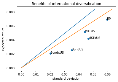
9.2.4. Two mean-variance frontiers: For domestic and Global investors#

We will now plot the two frontiers together with the underlying assets

# # Lets visualize this in a plot including the two investment frontiers

# # set different expected return targets
# mu_target=np.linspace(0,0.1/12,20)
# # international portfolios

# plt.plot(mu_target/SR_int,mu_target)

# #Domestic portfolios
# plt.plot(mu_target/SR_dom,mu_target)
# #Individual assets
# plt.xlabel('standard deviation')
# plt.ylabel('expected return')
# plt.title('Benefits of international diversification')
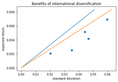
# plt.scatter(Re.std(),Re.mean())

<matplotlib.collections.PathCollection at 0x216674229a0>

Lets add label to the dots so we know which asset corresponds to each point

For that I will run the same code above and add a for loop that lopps though the column name of the Re dataframe and uses the text functio to write the column name in the correct position where the x-dimension is the asset volatility and y-dimension is the asset avereage return

# mu_target=np.linspace(0,0.1/12,20)
# plt.plot(mu_target/SR_int,mu_target)
# plt.plot(mu_target/SR_dom,mu_target)
# plt.scatter(Re.std(),Re.mean())

# plt.xlabel('standard deviation')
# plt.ylabel('expected return')
# plt.title('Benefits of international diversification')
# # lets add some labels so we know which point is each portfolio


# for label in Re.columns :
#    plt.text(Re.std()[label],Re.mean()[label],label)

Quantitative Investing

Case study on international portfolio diversification

Contents

9.2. Case study on international portfolio diversification#

9.2.1. Targeting desired Voaltiltiy#

9.2.2. Targeting Desired Expected Return#

9.2.3. Domestic Tangency Portfolio#

9.2.4. Two mean-variance frontiers: For domestic and Global investors#