5.2. Basic Functionality#

5.2.1. Industry portfolios data#

In this lecture, we will use industry portfolio data by industry at a monthly frequency.

those are portfolio of stocks of firms in different sectors of the economy

import pandas as pd

%matplotlib inline

First, we will download the data directly from a url and read it into a pandas DataFrame.

## Load up the data -- this will take a couple seconds
url = "https://raw.githubusercontent.com/amoreira2/Lectures/main/assets/data/49_Industry_Portfolios.CSV"
industret_raw = pd.read_csv(url, parse_dates=["Date"])

The pandas read_csv will determine most datatypes of the underlying columns. The exception here is that we need to give pandas a hint so it can load up the Date column as a Python datetime type: the parse_dates=["Date"].

We can see the basic structure of the downloaded data by getting the first 5 rows, which directly matches the underlying CSV file.

industret_raw.head()

	Date	industry	returns	nfirms	size
0	1926-07-31	Agric	2.37	3	99.80
1	1926-07-31	Food	0.12	40	31.19
2	1926-07-31	Soda	-99.99	0	-99.99
3	1926-07-31	Beer	-5.19	3	7.12
4	1926-07-31	Smoke	1.29	16	59.72

Note that a row has a date, industry , returns, number of firms in the portfolio and average size of the firm.

Note also the -99.99 which in this case is code for missing observation

For our analysis, we want to look at the firm size across different industries over time, which requires a transformation of the data similar to an Excel pivot-table.

# Don't worry about the details here quite yet
size_all = (
    industret_raw
    .reset_index()
    .pivot_table(index="Date", columns="industry", values="size")
)
size_all.head()

industry	Aero	Agric	Autos	Banks	Beer	BldMt	Books	Boxes	BusSv	Chems	...	Smoke	Soda	Softw	Steel	Telcm	Toys	Trans	Txtls	Util	Whlsl
Date
1926-07-31	9.52	99.80	47.55	14.50	7.12	20.80	4.33	35.35	11.21	57.59	...	59.72	-99.99	-99.99	48.56	350.36	13.00	68.67	5.78	81.22	1.19
1926-08-31	9.46	102.06	55.11	15.17	6.75	21.30	6.50	37.86	11.81	62.13	...	60.47	-99.99	-99.99	50.39	353.27	14.12	69.79	5.79	86.81	0.90
1926-09-30	8.78	104.34	57.11	16.97	8.58	22.27	9.29	36.82	11.99	65.53	...	64.03	-99.99	-99.99	51.21	360.96	16.50	72.90	6.25	85.01	0.95
1926-10-31	8.15	102.91	59.69	16.46	8.92	22.04	8.83	34.77	12.01	68.47	...	64.42	-99.99	-99.99	51.02	364.16	17.88	72.71	6.36	86.41	0.88
1926-11-30	7.07	102.34	54.81	14.52	8.62	21.05	9.31	32.80	12.17	65.06	...	65.08	-99.99	-99.99	48.90	363.74	17.62	70.58	6.38	83.92	0.74

5 rows × 49 columns

size_all.columns

Index(['Aero ', 'Agric', 'Autos', 'Banks', 'Beer ', 'BldMt', 'Books', 'Boxes',
       'BusSv', 'Chems', 'Chips', 'Clths', 'Cnstr', 'Coal ', 'Drugs', 'ElcEq',
       'FabPr', 'Fin  ', 'Food ', 'Fun  ', 'Gold ', 'Guns ', 'Hardw', 'Hlth ',
       'Hshld', 'Insur', 'LabEq', 'Mach ', 'Meals', 'MedEq', 'Mines', 'Oil  ',
       'Other', 'Paper', 'PerSv', 'RlEst', 'Rtail', 'Rubbr', 'Ships', 'Smoke',
       'Soda ', 'Softw', 'Steel', 'Telcm', 'Toys ', 'Trans', 'Txtls', 'Util ',
       'Whlsl'],
      dtype='object', name='industry')

Finally, we can filter it to look at a subset of the columns (i.e. “industry” in this case).

industries = [
    "Autos","Banks", "Meals", "Softw",
    "Smoke", "Telcm", "Mines"
]
size = size_all[industries]
size.tail()

industry	Autos	Banks	Meals	Softw	Smoke	Telcm	Mines
Date
2020-11-30	11504.82	5372.76	8638.65	22509.62	59424.37	20127.11	7379.30
2020-12-31	15667.02	6344.33	9595.61	24701.31	64210.14	23242.82	8377.75
2021-01-31	18292.42	6813.01	9983.06	25503.86	68622.27	24468.39	9186.89
2021-02-28	20561.46	6581.58	9531.13	25834.04	67059.98	23911.24	9376.07
2021-03-31	18531.08	7511.02	10445.51	26799.04	70900.88	24972.99	10770.47

When plotting, a DataFrame knows the column and index names.

size.plot(figsize=(8, 6),logy=True)

<AxesSubplot:xlabel='Date'>

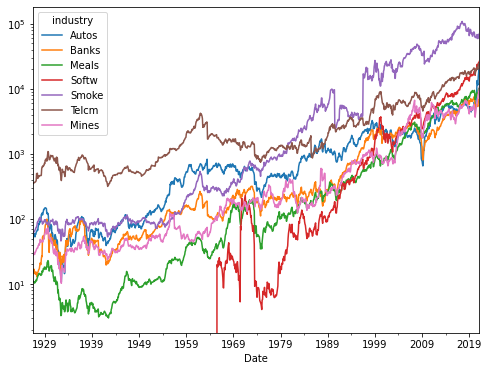
See exercise 1 in the exercise list

5.2.2. Dates in pandas#

You might have noticed that our index now has a nice format for the dates (YYYY-MM-DD) rather than just a year.

This is because the dtype of the index is a variant of datetime.

size.index

DatetimeIndex(['1926-07-31', '1926-08-31', '1926-09-30', '1926-10-31',
               '1926-11-30', '1926-12-31', '1927-01-31', '1927-02-28',
               '1927-03-31', '1927-04-30',
               ...
               '2020-06-30', '2020-07-31', '2020-08-31', '2020-09-30',
               '2020-10-31', '2020-11-30', '2020-12-31', '2021-01-31',
               '2021-02-28', '2021-03-31'],
              dtype='datetime64[ns]', name='Date', length=1137, freq=None)

We can index into a DataFrame with a DatetimeIndex using string representations of dates.

For example

# Data corresponding to a single date
size.loc["01/31/2000", :]

industry
Autos     2461.97
Banks     2249.50
Meals      800.97
Softw     3597.20
Smoke    12584.58
Telcm     8978.29
Mines      967.26
Name: 2000-01-31 00:00:00, dtype: float64

# Data for all days between New Years Day and June first in the year 2000
size.loc["01/31/2000":"06/30/2000", :]

industry	Autos	Banks	Meals	Softw	Smoke	Telcm	Mines
Date
2000-01-31	2461.97	2249.50	800.97	3597.20	12584.58	8978.29	967.26
2000-02-29	2504.11	2203.67	741.71	3270.95	11499.46	8739.86	955.71
2000-03-31	2290.96	1974.93	652.38	3603.68	11038.70	8463.58	881.00
2000-04-30	2545.41	2291.46	767.18	3733.34	11335.75	9098.77	938.08
2000-05-31	2873.71	2225.48	796.35	3050.85	14605.66	8217.91	865.02
2000-06-30	2458.02	2414.05	762.56	2740.98	17434.72	7235.48	871.13

We will learn more about what pandas can do with dates and times in an upcoming lecture on time series data.

5.2.3. DataFrame Aggregations#

Let’s talk about aggregations.

Loosely speaking, an aggregation is an operation that combines multiple values into a single value.

For example, computing the mean of three numbers (for example [0, 1, 2]) returns a single number (1).

We will use aggregations extensively as we analyze and manipulate our data.

Thankfully, pandas makes this easy!

5.2.3.1. Built-in Aggregations#

pandas already has some of the most frequently used aggregations.

For example:

Mean (mean)
Variance (var)
Standard deviation (std)
Minimum (min)
Median (median)
Maximum (max)
etc…

Note

When looking for common operations, using “tab completion” goes a long way.

size.mean()

industry
Autos     1271.677274
Banks      952.728619
Meals      984.425286
Softw     1550.233544
Smoke    12058.789384
Telcm     3468.995172
Mines      970.964626
dtype: float64

As seen above, the aggregation’s default is to aggregate each column.

However, by using the axis keyword argument, you can do aggregations by row as well.

size.var(axis=1).head()

Date
1926-07-31    19263.014148
1926-08-31    19496.461081
1926-09-30    20222.654548
1926-10-31    20548.252614
1926-11-30    20565.567314
dtype: float64

Note that below min and max are not in quotes becasue these are functions defined in python enviroment, while mean and std are in quotes because they are methods of the dataframe.

min and max are objects that python understand in general, while mean and std it only understands in the context of the dataframe.

size.agg([min, max,'mean','std'])

	Autos	Banks	Meals	Softw	Smoke	Telcm	Mines
min	10.790000	13.000000	3.010000	-99.990000	45.980000	317.100000	10.270000
max	20561.460000	7548.840000	10445.510000	26799.040000	109069.340000	24972.990000	10770.470000
mean	1271.677274	952.728619	984.425286	1550.233544	12058.789384	3468.995172	970.964626
std	1899.907582	1566.005467	2027.328596	3831.668701	22297.623981	4569.770894	1702.291519

5.2.4. Transforms#

Many analytical operations do not necessarily involve an aggregation.

The output of a function applied to a Series might need to be a new Series.

Some examples:

Compute the percentage change in average firm size from month to month.
Calculate the cumulative sum of elements in each column.

5.2.4.1. Built-in Transforms#

pandas comes with many transform functions including:

Cumulative sum/max/min/product (cum(sum|min|max|prod))
Difference (diff)
Elementwise addition/subtraction/multiplication/division (+, -, *, /)
Percent change (pct_change)
Number of occurrences of each distinct value (value_counts)
Absolute value (abs)

Again, tab completion is helpful when trying to find these functions.

size.head()

industry	Autos	Banks	Meals	Softw	Smoke	Telcm	Mines
Date
1926-07-31	47.55	14.50	10.82	-99.99	59.72	350.36	27.74
1926-08-31	55.11	15.17	11.00	-99.99	60.47	353.27	29.30
1926-09-30	57.11	16.97	10.94	-99.99	64.03	360.96	29.45
1926-10-31	59.69	16.46	10.80	-99.99	64.42	364.16	29.46
1926-11-30	54.81	14.52	10.33	-99.99	65.08	363.74	28.51

size.pct_change().head()

industry	Autos	Banks	Meals	Softw	Smoke	Telcm	Mines
Date
1926-07-31	NaN	NaN	NaN	NaN	NaN	NaN	NaN
1926-08-31	0.158991	0.046207	0.016636	0.0	0.012559	0.008306	0.056236
1926-09-30	0.036291	0.118655	-0.005455	0.0	0.058872	0.021768	0.005119
1926-10-31	0.045176	-0.030053	-0.012797	0.0	0.006091	0.008865	0.000340
1926-11-30	-0.081756	-0.117861	-0.043519	0.0	0.010245	-0.001153	-0.032247

size.diff().head()

industry	Autos	Banks	Meals	Softw	Smoke	Telcm	Mines
Date
1926-07-31	NaN	NaN	NaN	NaN	NaN	NaN	NaN
1926-08-31	7.56	0.67	0.18	0.0	0.75	2.91	1.56
1926-09-30	2.00	1.80	-0.06	0.0	3.56	7.69	0.15
1926-10-31	2.58	-0.51	-0.14	0.0	0.39	3.20	0.01
1926-11-30	-4.88	-1.94	-0.47	0.0	0.66	-0.42	-0.95

Transforms can be split into to several main categories:

Series transforms: functions that take in one Series and produce another Series. The index of the input and output does not need to be the same.
Scalar transforms: functions that take a single value and produce a single value. An example is the abs method, or adding a constant to each value of a Series.

5.2.4.2. Custom Series Transforms#

pandas also simplifies applying custom Series transforms to a Series or the columns of a DataFrame. The steps are:

Write a Python function that takes a Series and outputs a new Series.
Pass our new function as an argument to the apply method (alternatively, the transform method).

As an example, we will standardize our return data to have mean 0 and standard deviation 1.

After doing this, we can use an aggregation to determine at which date the return is most different from “normal times” for each industry.

# lets now work with the return data

returns_all = (
    industret_raw
    .reset_index()
    .pivot_table(index="Date", columns="industry", values="returns")
)

returns = returns_all[industries]
returns.head()

industry	Autos	Banks	Meals	Softw	Smoke	Telcm	Mines
Date
1926-07-31	16.39	4.61	1.87	-99.99	1.29	0.83	5.64
1926-08-31	4.23	11.83	-0.13	-99.99	6.50	2.17	0.55
1926-09-30	4.83	-1.75	-0.56	-99.99	1.26	2.41	1.74
1926-10-31	-7.93	-11.82	-4.11	-99.99	1.06	-0.11	-3.20
1926-11-30	-0.66	-2.97	4.33	-99.99	4.55	1.63	8.46

#
# Step 1: We write the Series transform function that we'd like to use
#
def standardize_data(x):
    """
    Changes the data in a Series to become mean 0 with standard deviation 1
    """
    mu = x.mean()
    std = x.std()

    return (x - mu)/std

#
# Step 2: Apply our function via the apply method.
#
std_returns = returns.apply(standardize_data)
std_returns.head()

industry	Autos	Banks	Meals	Softw	Smoke	Telcm	Mines
Date
1926-07-31	1.849843	0.488467	0.121700	-1.177902	0.025602	-0.007572	0.632371
1926-08-31	0.370785	1.512875	-0.186634	-1.177902	0.920361	0.283083	-0.066595
1926-09-30	0.443765	-0.413921	-0.252926	-1.177902	0.020450	0.335140	0.096817
1926-10-31	-1.108273	-1.842701	-0.800219	-1.177902	-0.013898	-0.211464	-0.581551
1926-11-30	-0.224001	-0.587020	0.500951	-1.177902	0.585470	0.165953	1.019618

# Takes the absolute value of all elements of a function
abs_std_returns = std_returns.abs()

abs_std_returns.head()

industry	Autos	Banks	Meals	Softw	Smoke	Telcm	Mines
Date
1926-07-31	1.849843	0.488467	0.121700	1.177902	0.025602	0.007572	0.632371
1926-08-31	0.370785	1.512875	0.186634	1.177902	0.920361	0.283083	0.066595
1926-09-30	0.443765	0.413921	0.252926	1.177902	0.020450	0.335140	0.096817
1926-10-31	1.108273	1.842701	0.800219	1.177902	0.013898	0.211464	0.581551
1926-11-30	0.224001	0.587020	0.500951	1.177902	0.585470	0.165953	1.019618

# find the date when returns was "most different from normal" for each industry
def idxmax(x):
    # idxmax of Series will return index of maximal value
    return x.idxmax()

abs_std_returns.agg(idxmax)

industry
Autos   1933-04-30
Banks   1933-04-30
Meals   1973-11-30
Softw   1970-09-30
Smoke   1933-04-30
Telcm   1932-08-31
Mines   1932-07-31
dtype: datetime64[ns]

5.2.5. Boolean Selection#

We have seen how we can select subsets of data by referring to the index or column names.

However, we often want to select based on conditions met by the data itself.

Some examples are:

Restrict analysis to all individuals older than 18.
Look at data that corresponds to particular time periods.
Analyze only data that corresponds to a recession.
Obtain data for a specific product or customer ID.

We will be able to do this by using a Series or list of boolean values to index into a Series or DataFrame.

Let’s look at some examples.

size_small = size.head()  # Create smaller data so we can see what's happening
size_small

industry	Autos	Banks	Meals	Softw	Smoke	Telcm	Mines
Date
1926-07-31	47.55	14.50	10.82	-99.99	59.72	350.36	27.74
1926-08-31	55.11	15.17	11.00	-99.99	60.47	353.27	29.30
1926-09-30	57.11	16.97	10.94	-99.99	64.03	360.96	29.45
1926-10-31	59.69	16.46	10.80	-99.99	64.42	364.16	29.46
1926-11-30	54.81	14.52	10.33	-99.99	65.08	363.74	28.51

# list of booleans selects rows
size_small.loc[[True, True, True, False, False]]

industry	Autos	Banks	Meals	Softw	Smoke	Telcm	Mines
Date
1926-07-31	47.55	14.50	10.82	-99.99	59.72	350.36	27.74
1926-08-31	55.11	15.17	11.00	-99.99	60.47	353.27	29.30
1926-09-30	57.11	16.97	10.94	-99.99	64.03	360.96	29.45

# second argument selects columns, the  ``:``  means "all".
# here we use it to select all columns
size_small.loc[[True, False, True, False, True], :]

industry	Autos	Banks	Meals	Softw	Smoke	Telcm	Mines
Date
1926-07-31	47.55	14.50	10.82	-99.99	59.72	350.36	27.74
1926-09-30	57.11	16.97	10.94	-99.99	64.03	360.96	29.45
1926-11-30	54.81	14.52	10.33	-99.99	65.08	363.74	28.51

# can use booleans to select both rows and columns
size_small.loc[[True, True, True, False, False], [True, False, False, False, False, True, True]]

industry	Autos	Telcm	Mines
Date
1926-07-31	47.55	350.36	27.74
1926-08-31	55.11	353.27	29.30
1926-09-30	57.11	360.96	29.45

5.2.5.1. Creating Boolean DataFrames/Series#

We can use conditional statements to construct Series of booleans from our data.

size_small["Autos"] <55

Date
1926-07-31     True
1926-08-31    False
1926-09-30    False
1926-10-31    False
1926-11-30     True
Name: Autos, dtype: bool

Once we have our Series of bools, we can use it to extract subsets of rows from our DataFrame.

size_small.loc[size_small["Autos"] < 55]

industry	Autos	Banks	Meals	Softw	Smoke	Telcm	Mines
Date
1926-07-31	47.55	14.50	10.82	-99.99	59.72	350.36	27.74
1926-11-30	54.81	14.52	10.33	-99.99	65.08	363.74	28.51

size_small["Banks"] > size_small["Autos"]

Date
1926-07-31    False
1926-08-31    False
1926-09-30    False
1926-10-31    False
1926-11-30    False
dtype: bool

big_Autos = size_small["Autos"] > size_small["Banks"]
size_small.loc[big_Autos]

industry	Autos	Banks	Meals	Softw	Smoke	Telcm	Mines
Date
1926-07-31	47.55	14.50	10.82	-99.99	59.72	350.36	27.74
1926-08-31	55.11	15.17	11.00	-99.99	60.47	353.27	29.30
1926-09-30	57.11	16.97	10.94	-99.99	64.03	360.96	29.45
1926-10-31	59.69	16.46	10.80	-99.99	64.42	364.16	29.46
1926-11-30	54.81	14.52	10.33	-99.99	65.08	363.74	28.51

5.2.5.1.1. Multiple Conditions#

In the boolean section of the basics lecture, we saw that we can use the words and and or to combine multiple booleans into a single bool.

Recall:

True and False -> False
True and True -> True
False and False -> False
True or False -> True
True or True -> True
False or False -> False

We can do something similar in pandas, but instead of bool1 and bool2 we write:

(bool_series1) & (bool_series2)

Likewise, instead of bool1 or bool2 we write:

(bool_series1) | (bool_series2)

small_BksAut = (size_small["Banks"] < 15) & (size_small["Autos"] < 56)
small_BksAut

Date
1926-07-31     True
1926-08-31    False
1926-09-30    False
1926-10-31    False
1926-11-30     True
dtype: bool

size_small[small_BksAut]

industry	Autos	Banks	Meals	Softw	Smoke	Telcm	Mines
Date
1926-07-31	47.55	14.50	10.82	-99.99	59.72	350.36	27.74
1926-11-30	54.81	14.52	10.33	-99.99	65.08	363.74	28.51

5.2.5.1.2. `isin`#

Sometimes, we will want to check whether a data point takes on one of a several fixed values.

We could do this by writing (df["x"] == val_1) | (df["x"] == val_2) (like we did above), but there is a better way: the .isin method

size_small["Smoke"].isin([60.47, 64.42])

Date
1926-07-31    False
1926-08-31     True
1926-09-30    False
1926-10-31     True
1926-11-30    False
Name: Smoke, dtype: bool

# now select full rows where this Series is True
size_small.loc[size_small["Smoke"].isin([60.47, 64.42])]

industry	Autos	Banks	Meals	Softw	Smoke	Telcm	Mines
Date
1926-08-31	55.11	15.17	11.0	-99.99	60.47	353.27	29.30
1926-10-31	59.69	16.46	10.8	-99.99	64.42	364.16	29.46

5.2.5.1.3. `.any` and `.all`#

Recall from the boolean section of the basics lecture that the Python functions any and all are aggregation functions that take a collection of booleans and return a single boolean.

any returns True whenever at least one of the inputs are True while all is True only when all the inputs are True.

Series and DataFrames with dtype bool have .any and .all methods that apply this logic to pandas objects.

Let’s use these methods to count how many months all the states in our sample had low returns.

As we work through this example, consider the [“want operator”], a helpful concept from Nobel Laureate Tom Sargent for clearly stating the goal of our analysis and determining the steps necessary to reach the goal.

We always begin by writing Want: followed by what we want to accomplish.

In this case, we would write:

Want: Count the number of months in which all industries in our sample had returns less than -5%

After identifying the want, we work backwards to identify the steps necessary to accomplish our goal.

So, starting from the result, we have:

Sum the number of True values in a Series indicating dates for which all industries had low returns.
Build the Series used in the last step by using the .all method on a DataFrame containing booleans indicating whether each industry had low returns at each date.
Build the DataFrame used in the previous step using a < comparison.

Now that we have a clear plan, let’s follow through and apply the want operator:

# Step 3: construct the DataFrame of bools
low = returns_all < -5
low.head()

industry	Aero	Agric	Autos	Banks	Beer	BldMt	Books	Boxes	BusSv	Chems	...	Smoke	Soda	Softw	Steel	Telcm	Toys	Trans	Txtls	Util	Whlsl
Date
1926-07-31	False	False	False	False	True	False	False	False	False	False	...	False	True	True	False	False	False	False	False	False	True
1926-08-31	True	False	False	False	False	False	False	False	False	False	...	False	True	True	False	False	False	False	False	False	False
1926-09-30	True	False	False	False	False	False	False	True	False	False	...	False	True	True	False	False	False	False	False	False	True
1926-10-31	True	False	True	True	False	False	False	True	False	False	...	False	True	True	False	False	False	False	False	False	True
1926-11-30	False	False	False	False	False	False	True	False	False	False	...	False	True	True	False	False	False	False	False	False	False

5 rows × 49 columns

# Step 2: use the .all method on axis=1 to get the dates where all states have a True
all_low = low.all(axis=1)
all_low.head()

Date
1926-07-31    False
1926-08-31    False
1926-09-30    False
1926-10-31    False
1926-11-30    False
dtype: bool

# Step 1: Call .sum to add up the number of True values in `all_low`
#         (note that True == 1 and False == 0 in Python, so .sum will count Trues)


print(f'Out of {len(all_low)} months, {all_low.sum()} had low returns across all industries')

Out of 1137 months, 5 had low returns across all industries

Quantitative Investing

Basic Functionality

Contents

5.2. Basic Functionality#

5.2.1. Industry portfolios data#

5.2.2. Dates in pandas#

5.2.3. DataFrame Aggregations#

5.2.3.1. Built-in Aggregations#

5.2.4. Transforms#

5.2.4.1. Built-in Transforms#

5.2.4.2. Custom Series Transforms#

5.2.5. Boolean Selection#

5.2.5.1. Creating Boolean DataFrames/Series#

5.2.5.1.1. Multiple Conditions#

5.2.5.1.2. `isin`#

5.2.5.1.3. `.any` and `.all`#

Quantitative Investing

Basic Functionality

Contents

5.2. Basic Functionality#

5.2.1. Industry portfolios data#

5.2.2. Dates in pandas#

5.2.3. DataFrame Aggregations#

5.2.3.1. Built-in Aggregations#

5.2.4. Transforms#

5.2.4.1. Built-in Transforms#

5.2.4.2. Custom Series Transforms#

5.2.5. Boolean Selection#

5.2.5.1. Creating Boolean DataFrames/Series#

5.2.5.1.1. Multiple Conditions#

5.2.5.1.2. isin#

5.2.5.1.3. .any and .all#

5.2.5.1.2. `isin`#

5.2.5.1.3. `.any` and `.all`#