
Exercises#
Scientific/Numpy#
Exercises#
NEED TO CHECK IN exercises are approproiate
Try indexing into another element of your choice from the 3-dimensional array.
Building an understanding of indexing means working through this type of operation several times – without skipping steps!
Exercise 2
Look at the 2-dimensional array x_2d.
Does the inner-most index correspond to rows or columns? What does the outer-most index correspond to?
Write your thoughts.
Exercise 3
What would you do to extract the array [[5, 6], [50, 60]]?
Exercise 4
Do you recall what multiplication by an integer did for lists?
How does this differ?
Exercise 5
Let’s revisit a bond pricing example we saw in Control flow.
Recall that the equation for pricing a bond with coupon payment \( C \), face value \( M \), yield to maturity \( i \), and periods to maturity \( N \) is
In the code cell below, we have defined variables for i, M and C.
You have two tasks:
Define a numpy array
Nthat contains all maturities between 1 and 10 (hint look at thenp.arangefunction).Using the equation above, determine the bond prices of all maturity levels in your array.
i = 0.03
M = 100
C = 5

# Define array here

# price bonds here
Exercise 1#
Consider the polynomial expression
$\( p(x) = a_0 + a_1 x + a_2 x^2 + \cdots a_N x^N = \sum_{n=0}^N a_n x^n \tag{1} \)$
Earlier, you wrote a simple function p(x, coeff) to evaluate (9.1) without considering efficiency.
Now write a new function that does the same job, but uses NumPy arrays and array operations for its computations, rather than any form of Python loop.
(Such functionality is already implemented as np.poly1d, but for the sake of the exercise don’t use this class)
Hint: Use
np.cumprod()
Exercise 2#
Let q be a NumPy array of length n with q.sum() == 1.
Plotting#
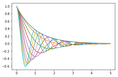
Exercise 1#
Plot the function
over the interval \( [0, 5] \) for each \( \theta \) in np.linspace(0, 2, 10).
Place all the curves in the same figure.
The output should look like this
Linear algebra#
Exercises#
Alice is a stock broker who owns two types of assets: A and B. She owns 100 units of asset A and 50 units of asset B. The current interest rate is 5%. Each of the A assets have a remaining duration of 6 years and pay \\(1500 each year, while each of the B assets have a remaining duration of 4 years and pay \\\)500 each year. Alice would like to retire if she can sell her assets for more than \$500,000. Use vector addition, scalar multiplication, and dot products to determine whether she can retire.
Exercise 2
Which of the following operations will work and which will create errors because of size issues?
Test out your intuitions in the code cell below
x1 @ x2
x2 @ x1
x2 @ x3
x3 @ x2
x1 @ x3
x4 @ y1
x4 @ y2
y1 @ x4
y2 @ x4
# testing area
Exercise 3
Compare the distribution above to the final values of a long simulation.
If you multiply the distribution by 1,000,000 (the number of workers), do you get (roughly) the same number as the simulation?
# your code here
Randomness#
Exercises#
EDIT EXERCISESS
Wikipedia and other credible statistics sources tell us that the mean and variance of the Uniform(0, 1) distribution are (1/2, 1/12) respectively.
How could we check whether the numpy random numbers approximate these values?
Exercise 2
Some execise
# your code here
Exercise 3
Assume you have been given the opportunity to choose between one of three financial assets:
You will be given the asset for free, allowed to hold it indefinitely, and keeping all payoffs.
Also assume the assets’ payoffs are distributed as follows:
Normal with \( \mu = 10, \sigma = 5 \)
Gamma with \( k = 5.3, \theta = 2 \)
Gamma with \( k = 5, \theta = 2 \)
Use scipy.stats to answer the following questions:
Which asset has the highest average returns?
Which asset has the highest median returns?
Which asset has the lowest coefficient of variation (standard deviation divided by mean)?
Which asset would you choose? Why? (Hint: There is not a single right answer here. Be creative and express your preferences)
# your code here
Pandas#
Intro#
Exercises#
For each of the following exercises, we recommend reading the documentation for help.
Display only the first 2 elements of the Series using the
.headmethod.Using the
plotmethod, make a bar plot.Use
.locto select the lowest/highest unemployment rate shown in the Series.Run the code
unemp.dtypebelow. What does it give you? Where do you think it comes from?
Exercise 2
For each of the following, we recommend reading the documentation for help.
Use introspection (or google-fu) to find a way to obtain a list with all of the column names in
unemp_region.Using the
plotmethod, make a bar plot. What does it look like now?Use
.locto select the the unemployment data for theNorthEastandWestfor the years 1995, 2005, 2011, and 2015.Run the code
unemp_region.dtypesbelow. What does it give you? How does this compare withunemp.dtype?
BASICS#
Exercises#
Looking at the displayed DataFrame above, can you identify the index? The columns?
You can use the cell below to verify your visual intuition.
# your code here
Exercise 2
Do the following exercises in separate code cells below:
At each date, what is the minimum unemployment rate across all states in our sample?
What was the median unemployment rate in each state?
What was the maximum unemployment rate across the states in our sample? What state did it happen in? In what month/year was this achieved?
Hint 1: What Python type (not
dtype) is returned by the aggregation?Hint 2: Read documentation for the method
idxmax
Classify each state as high or low volatility based on whether the variance of their unemployment is above or below 4.
# min unemployment rate by state
# median unemployment rate by state
# max unemployment rate across all states and Year
# low or high volatility
Exercise 3
Imagine that we want to determine whether unemployment was high (> 6.5), medium (4.5 < x <= 6.5), or low (<= 4.5) for each state and each month.
Write a Python function that takes a single number as an input and outputs a single string noting if that number is high, medium, or low.
Pass your function to
applymap(quiz: whyapplymapand notaggorapply?) and save the result in a new DataFrame calledunemp_bins.(Challenging) This exercise has multiple parts:
Use another transform on
unemp_binsto count how many times each state had each of the three classifications.
- Hint 1: Will this value counting function be a Series or scalar transform?
- Hint 2: Try googling “pandas count unique value” or something similar to find the right transform.Construct a horizontal bar chart of the number of occurrences of each level with one bar per state and classification (21 total bars).
(Challenging) Repeat the previous step, but count how many states had each classification in each month. Which month had the most states with high unemployment? What about medium and low?
# Part 1: Write a Python function to classify unemployment levels.
# Part 2: Pass your function from part 1 to applymap
unemp_bins = unemp.applymap#replace this comment with your code!!
# Part 3: Count the number of times each state had each classification.

## then make a horizontal bar chart here
# Part 4: Apply the same transform from part 4, but to each date instead of to each state.
Exercise 4
For a single state of your choice, determine what the mean unemployment is during “Low”, “Medium”, and “High” unemployment times (recall your
unemp_binsDataFrame from the exercise above).Think about how you would do this for all the states in our sample and write your thoughts… We will soon learn tools that will greatly simplify operations like this that operate on distinct groups of data at a time.
Which states in our sample performs the best during “bad times?” To determine this, compute the mean unemployment for each state only for months in which the mean unemployment rate in our sample is greater than 7.
tHE INDEX#
Exercises#
What happens when you apply the mean method to im_ex_tiny?
In particular, what happens to columns that have missing data? (HINT:
also looking at the output of the sum method might help)
Exercise 2
For each of the examples below do the following:
Determine which of the rules above applies.
Identify the
typeof the returned value.Explain why the slicing operation returned the data it did.
Write your answers.
wdi.loc[["United States", "Canada"]]
| GovExpend | Consumption | Exports | Imports | GDP | ||
|---|---|---|---|---|---|---|
| country | year | |||||
| Canada | 2017 | 0.372665 | 1.095475 | 0.582831 | 0.600031 | 1.868164 |
| 2016 | 0.364899 | 1.058426 | 0.576394 | 0.575775 | 1.814016 | |
| 2015 | 0.358303 | 1.035208 | 0.568859 | 0.575793 | 1.794270 | |
| 2014 | 0.353485 | 1.011988 | 0.550323 | 0.572344 | 1.782252 | |
| 2013 | 0.351541 | 0.986400 | 0.518040 | 0.558636 | 1.732714 | |
| 2012 | 0.354342 | 0.961226 | 0.505969 | 0.547756 | 1.693428 | |
| 2011 | 0.351887 | 0.943145 | 0.492349 | 0.528227 | 1.664240 | |
| 2010 | 0.347332 | 0.921952 | 0.469949 | 0.500341 | 1.613543 | |
| 2009 | 0.339686 | 0.890078 | 0.440692 | 0.439796 | 1.565291 | |
| 2008 | 0.330766 | 0.889602 | 0.506350 | 0.502281 | 1.612862 | |
| 2007 | 0.318777 | 0.864012 | 0.530453 | 0.498002 | 1.596876 | |
| 2006 | 0.311382 | 0.827643 | 0.524461 | 0.470931 | 1.564608 | |
| 2005 | 0.303043 | 0.794390 | 0.519950 | 0.447222 | 1.524608 | |
| 2004 | 0.299854 | 0.764357 | 0.508657 | 0.416754 | 1.477317 | |
| 2003 | 0.294335 | 0.741796 | 0.481993 | 0.384199 | 1.433089 | |
| 2002 | 0.286094 | 0.721974 | 0.490465 | 0.368615 | 1.407725 | |
| 2001 | 0.279767 | 0.694230 | 0.484696 | 0.362023 | 1.366590 | |
| 2000 | 0.270553 | 0.677713 | 0.499526 | 0.380823 | 1.342805 | |
| United States | 2017 | 2.405743 | 12.019266 | 2.287071 | 3.069954 | 17.348627 |
| 2016 | 2.407981 | 11.722133 | 2.219937 | 2.936004 | 16.972348 | |
| 2015 | 2.373130 | 11.409800 | 2.222228 | 2.881337 | 16.710459 | |
| 2014 | 2.334071 | 11.000619 | 2.209555 | 2.732228 | 16.242526 | |
| 2013 | 2.353381 | 10.687214 | 2.118639 | 2.600198 | 15.853796 | |
| 2012 | 2.398873 | 10.534042 | 2.045509 | 2.560677 | 15.567038 | |
| 2011 | 2.434378 | 10.378060 | 1.978083 | 2.493194 | 15.224555 | |
| 2010 | 2.510143 | 10.185836 | 1.846280 | 2.360183 | 14.992053 | |
| 2009 | 2.507390 | 10.010687 | 1.646432 | 2.086299 | 14.617299 | |
| 2008 | 2.407771 | 10.137847 | 1.797347 | 2.400349 | 14.997756 | |
| 2007 | 2.351987 | 10.159387 | 1.701096 | 2.455016 | 15.018268 | |
| 2006 | 2.314957 | 9.938503 | 1.564920 | 2.395189 | 14.741688 | |
| 2005 | 2.287022 | 9.643098 | 1.431205 | 2.246246 | 14.332500 | |
| 2004 | 2.267999 | 9.311431 | 1.335978 | 2.108585 | 13.846058 | |
| 2003 | 2.233519 | 8.974708 | 1.218199 | 1.892825 | 13.339312 | |
| 2002 | 2.193188 | 8.698306 | 1.192180 | 1.804105 | 12.968263 | |
| 2001 | 2.112038 | 8.480461 | 1.213253 | 1.740797 | 12.746262 | |
| 2000 | 2.040500 | 8.272097 | 1.287739 | 1.790995 | 12.620268 |
wdi.loc[(["United States", "Canada"], [2010, 2011, 2012]), :]
| GovExpend | Consumption | Exports | Imports | GDP | ||
|---|---|---|---|---|---|---|
| country | year | |||||
| Canada | 2012 | 0.354342 | 0.961226 | 0.505969 | 0.547756 | 1.693428 |
| 2011 | 0.351887 | 0.943145 | 0.492349 | 0.528227 | 1.664240 | |
| 2010 | 0.347332 | 0.921952 | 0.469949 | 0.500341 | 1.613543 | |
| United States | 2012 | 2.398873 | 10.534042 | 2.045509 | 2.560677 | 15.567038 |
| 2011 | 2.434378 | 10.378060 | 1.978083 | 2.493194 | 15.224555 | |
| 2010 | 2.510143 | 10.185836 | 1.846280 | 2.360183 | 14.992053 |
wdi.loc["United States"]
| GovExpend | Consumption | Exports | Imports | GDP | |
|---|---|---|---|---|---|
| year | |||||
| 2017 | 2.405743 | 12.019266 | 2.287071 | 3.069954 | 17.348627 |
| 2016 | 2.407981 | 11.722133 | 2.219937 | 2.936004 | 16.972348 |
| 2015 | 2.373130 | 11.409800 | 2.222228 | 2.881337 | 16.710459 |
| 2014 | 2.334071 | 11.000619 | 2.209555 | 2.732228 | 16.242526 |
| 2013 | 2.353381 | 10.687214 | 2.118639 | 2.600198 | 15.853796 |
| 2012 | 2.398873 | 10.534042 | 2.045509 | 2.560677 | 15.567038 |
| 2011 | 2.434378 | 10.378060 | 1.978083 | 2.493194 | 15.224555 |
| 2010 | 2.510143 | 10.185836 | 1.846280 | 2.360183 | 14.992053 |
| 2009 | 2.507390 | 10.010687 | 1.646432 | 2.086299 | 14.617299 |
| 2008 | 2.407771 | 10.137847 | 1.797347 | 2.400349 | 14.997756 |
| 2007 | 2.351987 | 10.159387 | 1.701096 | 2.455016 | 15.018268 |
| 2006 | 2.314957 | 9.938503 | 1.564920 | 2.395189 | 14.741688 |
| 2005 | 2.287022 | 9.643098 | 1.431205 | 2.246246 | 14.332500 |
| 2004 | 2.267999 | 9.311431 | 1.335978 | 2.108585 | 13.846058 |
| 2003 | 2.233519 | 8.974708 | 1.218199 | 1.892825 | 13.339312 |
| 2002 | 2.193188 | 8.698306 | 1.192180 | 1.804105 | 12.968263 |
| 2001 | 2.112038 | 8.480461 | 1.213253 | 1.740797 | 12.746262 |
| 2000 | 2.040500 | 8.272097 | 1.287739 | 1.790995 | 12.620268 |
wdi.loc[("United States", 2010), ["GDP", "Exports"]]
GDP        14.992053
Exports     1.846280
Name: (United States, 2010), dtype: float64
wdi.loc[("United States", 2010)]
GovExpend       2.510143
Consumption    10.185836
Exports         1.846280
Imports         2.360183
GDP            14.992053
Name: (United States, 2010), dtype: float64
wdi.loc[[("United States", 2010), ("Canada", 2015)]]
| GovExpend | Consumption | Exports | Imports | GDP | ||
|---|---|---|---|---|---|---|
| country | year | |||||
| United States | 2010 | 2.510143 | 10.185836 | 1.846280 | 2.360183 | 14.992053 |
| Canada | 2015 | 0.358303 | 1.035208 | 0.568859 | 0.575793 | 1.794270 |
wdi.loc[["United States", "Canada"], "GDP"]
country        year
Canada         2017     1.868164
               2016     1.814016
               2015     1.794270
               2014     1.782252
               2013     1.732714
               2012     1.693428
               2011     1.664240
               2010     1.613543
               2009     1.565291
               2008     1.612862
               2007     1.596876
               2006     1.564608
               2005     1.524608
               2004     1.477317
               2003     1.433089
               2002     1.407725
               2001     1.366590
               2000     1.342805
United States  2017    17.348627
               2016    16.972348
               2015    16.710459
               2014    16.242526
               2013    15.853796
               2012    15.567038
               2011    15.224555
               2010    14.992053
               2009    14.617299
               2008    14.997756
               2007    15.018268
               2006    14.741688
               2005    14.332500
               2004    13.846058
               2003    13.339312
               2002    12.968263
               2001    12.746262
               2000    12.620268
Name: GDP, dtype: float64
wdi.loc["United States", "GDP"]
year
2017    17.348627
2016    16.972348
2015    16.710459
2014    16.242526
2013    15.853796
2012    15.567038
2011    15.224555
2010    14.992053
2009    14.617299
2008    14.997756
2007    15.018268
2006    14.741688
2005    14.332500
2004    13.846058
2003    13.339312
2002    12.968263
2001    12.746262
2000    12.620268
Name: GDP, dtype: float64
Exercise 3
Try setting my_df to some subset of the rows in wdi (use one of the
.loc variations above).
Then see what happens when you do wdi / my_df or my_df ** wdi.
Try changing the subset of rows in my_df and repeat until you
understand what is happening.
Exercise 4
Below, we create wdi2, which is the same as df4 except that the
levels of the index are swapped.
In the cells after df6 is defined, we have commented out
a few of the slicing examples from the previous exercise.
For each of these examples, use pd.IndexSlice to extract the same
data from df6.
(HINT: You will need to swap the order of the row slicing arguments
within the pd.IndexSlice.)
wdi2 = df.set_index(["year", "country"])
# wdi.loc["United States"]
# wdi.loc[(["United States", "Canada"], [2010, 2011, 2012]), :]
# wdi.loc[["United States", "Canada"], "GDP"]
Exercise 5
Use pd.IndexSlice to extract all data from wdiT where the year
level of the column names (the second level) is one of 2010, 2012, and 2014
Exercise 6
Look up the documentation for the reset_index method and study it to
learn how to do the following:
Move just the
yearlevel of the index back as a column.Completely throw away all levels of the index.
Remove the
countryof the index and do not keep it as a column.
# remove just year level and add as column
# throw away all levels of index
# Remove country from the index -- don't keep it as a column
Time Series#
Exercises#
By referring to table found at the link above, figure out the correct argument to
pass as format in order to parse the dates in the next three cells below.
Test your work by passing your format string to pd.to_datetime.
christmas_str2 = "2017:12:25"
dbacks_win = "M:11 D:4 Y:2001 9:15 PM"
america_bday = "America was born on July 4, 1776"
Exercise 2
Use pd.to_datetime to express the birthday of one of your friends
or family members as a datetime object.
Then use the strftime method to write a message of the format:
NAME's birthday is June 10, 1989 (a Saturday)
(where the name and date are replaced by the appropriate values)
Exercise 3
For each item in the list, extract the specified data from btc_usd:
July 2017 through August 2017 (inclusive)
April 25, 2015 to June 10, 2016
October 31, 2017
Exercise 4
Using the shift function, determine the week with the largest percent change
in the volume of trades (the "Volume (BTC)" column).
Repeat the analysis at the bi-weekly and monthly frequencies.
Hint 1: We have data at a daily frequency and one week is 7 days.
Hint 2: Approximate a month by 30 days.
# your code here
Exercise 5
Imagine that you have access to the DeLorean time machine from “Back to the Future”.
You are allowed to use the DeLorean only once, subject to the following conditions:
You may travel back to any day in the past.
On that day, you may purchase one bitcoin at market open.
You can then take the time machine 30 days into the future and sell your bitcoin at market close.
Then you return to the present, pocketing the profits.
How would you pick the day?
Think carefully about what you would need to compute to make the optimal choice. Try writing it out in the markdown cell below so you have a clear description of the want operator that we will apply after the exercise.
(Note: Don’t look too far below, because in the next non-empty cell we have written out our answer.)
To make this decision, we want to know …
Your answer here
Exercise 6
Do the following:
Write a pandas function that implements your strategy.
Pass it to the
aggmethod ofrolling_btc.Extract the
"Open"column from the result.Find the date associated with the maximum value in that column.
How much money did you make? Compare with your neighbor.
def daily_value(df):
    # DELETE `pass` below and replace it with your code
    pass

rolling_btc = btc_usd.rolling("30d")

# do steps 2-4 here
Exercise 7
Now suppose you still have access to the DeLorean, but the conditions are slightly different.
You may now:
Travel back to the first day of any month in the past.
On that day, you may purchase one bitcoin at market open.
You can then travel to any day in that month and sell the bitcoin at market close.
Then return to the present, pocketing the profits.
To which month would you travel? On which day of that month would you return to sell the bitcoin?
Discuss with your neighbor what you would need to compute to make the optimal choice. Try writing it out in the markdown cell below so you have a clear description of the want operator that we will apply after the exercise.
(Note: Don’t look too many cells below, because we have written out our answer.)
To make the optimal decision we need …
Your answer here
Exercise 8
Do the following:
Write a pandas function that implements your strategy.
Pass it to the
aggmethod ofresampled_btc.Extract the
"Open"column from the result.Find the date associated with the maximum value in that column.
How much money did you make? Compare with your neighbor.
Was this strategy more profitable than the previous one? By how much?
def monthly_value(df):
    # DELETE `pass` below and replace it with your code
    pass

resampled_btc = btc_usd.resample("MS")

# Do steps 2-4 here