
13.9. What Are Factors?#
Factors are characteristics or signals that help explain asset returns. They serve both as risk indicators and as return drivers. Academics emphasize their ability to explain expected returns and remove known sources of variation so that only “new” sources of alpha remain. Practitioners value them for improving performance measurement, risk management, and portfolio construction.
We can group factors based on what they aim to capture:
13.9.1. 🌍 Market & Sector Membership#
Market: Whether the asset belongs to a region (e.g., US, China). Encoded as 1 if present, 0 otherwise.
Sector: Broad industry grouping (e.g., tech, healthcare). Can be split into 5 to 100+ categories.
Works beyond equities—applicable to credit markets, bonds, etc.
These “membership” factors help isolate common shocks shared within countries or sectors.
13.9.2. 🧾 Accounting-Based Factors#
These aim to proxy for fundamentals and predict returns:
Value (Book-to-Market): Cheap stocks (high book relative to price) have historically earned higher returns. This remains one of the most studied and used factors in practice.
Profitability / Quality: Gross profitability (Revenue – COGS) / Assets helps separate high-quality stocks from deteriorating ones. Other signals include ROE, margins, earnings stability, accruals, and low debt levels.
Investment: Firms that invest less (e.g., low asset growth, low capital expenditures) tend to outperform, potentially because high investment reflects low marginal value or managerial empire-building.
Composite Quality Scores: Many practitioners combine profitability, stability, leverage, and growth into a single “quality” score for screening or weighting.
Combining quality with value is especially powerful: among firms with similar value metrics, those with high profitability tend to outperform.
13.9.3. 📉 Return-Based Factors#
These come from past return patterns and risk exposures:
Beta: Measures sensitivity to the market factor. The CAPM suggests a linear relation between beta and expected return, but empirically this relationship often breaks down.
Volatility: High total or idiosyncratic volatility is often associated with lower expected returns. Low-volatility stocks have outperformed in many global markets.
Short-Term Reversal: Stocks with very poor short-term performance tend to revert upwards, likely due to liquidity shocks, overreactions, or temporary flows.
Momentum: One of the strongest factors. Past 12-month return (excluding the most recent month) predicts future returns. Often interpreted as a proxy for underreaction or investor herding.
Skewness / Tail Risks: Assets with negatively skewed returns (lottery-like) may be overpriced due to behavioral demand.
13.9.4. 🔁 Trading-Based Factors#
These reflect investor behavior and flow-driven dynamics:
Short Interest: High short interest or high borrow cost signals pessimism and often predicts underperformance.
Active Ownership: Stocks targeted by activists or insiders tend to outperform, especially if tied to governance or restructuring.
Liquidity / Amihud Illiquidity: Illiquid stocks earn higher returns, possibly compensating for trading costs and risk.
Turnover / Share Issuance: High share issuance and high turnover have been linked to lower future returns, possibly reflecting overpricing.
Crowdedness matters: signals can lose predictive power when overused. Many trading-based factors capture frictions or flow-induced mispricing that decay with scale.
13.9.5. Final Note#
Even if a factor does not reliably predict expected returns, it may still explain co-movement across assets. That alone makes it essential for risk management and performance attribution. A robust understanding of both risk-based and behavioral interpretations helps in building resilient portfolios and separating true alpha from systematic exposure.
Below I have a broader discussion of some of these characteristics/investment strategies
13.9.6. 💼 Value Investing – Deep Dive#
Value investing is one of the most widely studied and implemented quantitative strategies.
13.9.6.1. 🔎 What is it?#
A strategy that tilts the portfolio toward stocks that appear cheap relative to a fundamental anchor—and away from those that appear expensive.
Mathematically: $\( W_t \propto \frac{F_t}{P_t} \)$ Where ( F_t ) is a proxy for a firm’s fundamental value and ( P_t ) is its price.
Common choices for ( F_t ):
Book Value
Earnings
Dividends
Cash Flows
Sales
This is the cross-sectional counterpart to time-series strategies that time the market based on aggregate valuation metrics like the dividend yield. However, cross-sectional value strategies tend to be more robust—even if they can underperform for long periods (as seen in the 2010s).
13.9.6.2. 📚 Academic Foundations#
Lakonishok, Shleifer, and Vishny (1994) : Behavioral view—investors overreact to past growth or bad news. Value stocks exploit these biases.
Fama and French (1996): Rational risk-based view—value stocks are riskier, consistent with multifactor models.
13.9.6.3. 🧠 Why Might It Work?#
1. Mispricing (Behavioral Story)
Investors extrapolate trends or overreact to news.
Growth stocks become overpriced (“glamorous”); value stocks are neglected (“ugly”).
Contrarian rebalancing can capture mean-reversion in sentiment.
2. Risk (Rational Story)
Value firms may be fundamentally riskier: more distress-prone, less flexible, or more sensitive to macro shocks.
This explains why value did poorly in crises like 2008 and 2020.
Empirical Challenge to CAPM:
In CAPM, higher expected return implies higher beta.
But as firms transition between value/growth portfolios, their beta doesn’t change accordingly.
This inconsistency suggests that beta alone can’t explain value spreads.
13.9.6.4. ⚖️ Summary#
Most researchers believe there’s a blend of both:
Behavioral elements (investor overreaction, underreaction, salience).
Risk-based explanations (distress risk, macro exposure).
Despite recent underperformance, value remains foundational in both academic research and institutional practice.
13.9.7. 📈 Return-Based Strategies#
Momentum is the tendency for stocks that have performed relatively well in the recent past to continue performing well in the near future—and likewise for recent underperformers. This is a cross-sectional phenomenon: it’s about relative strength across stocks, not absolute performance.
A classic momentum strategy buys recent winners and shorts recent losers. Over the 1963–1990 period, Jegadeesh and Titman (1993) showed that a strategy ranking stocks by past 6-to-12-month returns and taking long/short positions in the top/bottom deciles delivered abnormal returns of 12% per year.
13.9.7.1. ⚖️ Momentum vs. Value#
While value strategies buy beaten-down stocks based on fundamentals, momentum buys recent outperformers based on price trends. In fact, value and momentum often load on opposite ends of the performance spectrum:
Value stocks have low recent returns (hence low prices vs. fundamentals)
Momentum stocks have high recent returns (regardless of valuation)
13.9.7.2. 🛠️ How to Construct a Momentum Portfolio#
Daniel and Moskowitz (2015) provide a standard implementation:
Rank stocks based on cumulative returns from t–12 to t–2 months, skipping the most recent month to avoid short-term reversal effects. Select stocks in the top and bottom deciles to form long and short portfolios.
This 1-month skip is important to sidestep short-term noise and ensure the signal captures true momentum.
13.9.7.3. 🤔 Why Might It Work?#
Behavioral Explanation:
Investors are slow to fully process new information
News and sentiment get incorporated into prices gradually
Examples include political developments, earnings trends, or macro regime shifts (e.g., COVID, elections)
Rational Explanation:
Stocks with similar momentum may share exposure to unobserved risk factors
Momentum return could reflect compensation for time-varying risk exposures
However, it’s hard to find a well-defined risk factor that explains the magnitude and persistence of the momentum premium
Most academics lean toward behavioral explanations, though some admit rational risks may help explain co-movement.
⚠️ Caveat: Momentum crashes hard in high-volatility environments—notably in 2008 and 2020. So while profitable, it is not low risk.
13.9.7.4. 📚 Key Literature#
13.9.7.6. 📊 Empirical Evidence#
Below is a plot summarizing Sharpe ratios as a function of return lookback periods used for momentum signals:

🧪 Challenge: Can you reproduce this plot using CRSP data and simple momentum signal construction?
Momentum is one of the most powerful and puzzling return anomalies. Despite its risks, it remains central to many quantitative strategies and academic debates.
13.9.8. 🛡️ Defensive Investing#
Core idea:
Don’t chase high-return signals—target low-risk assets instead. Defensive investing is about recognizing that risk is more predictable than return and using that predictability to build superior portfolios.
“Why look for high-return assets if lower-risk ones consistently outperform on a risk-adjusted basis?”
13.9.8.1. 🤔 Motivation#
Traditional theory (e.g., CAPM) links higher expected return to higher beta.
But in the data, beta is not reliably compensated.
Instead, low-risk stocks often outperform high-risk ones on a risk-adjusted basis.
The tangency portfolio (true mean-variance optimal portfolio) is unobservable—real-world risk-return trade-offs may deviate from theory.
13.9.8.2. 📉 Three Key Low-Risk Anomalies#
13.9.8.2.1. 1. Betting Against Beta (BAB)#
Source: Frazzini & Pedersen (2014)
Strategy: Long low-beta stocks, short high-beta stocks, leverage up to equalize risk.
Empirical finding: Low-beta stocks earn high alphas, high-beta stocks earn very negative alphas.
📊 BAB Sharpe Ratio Evidence:
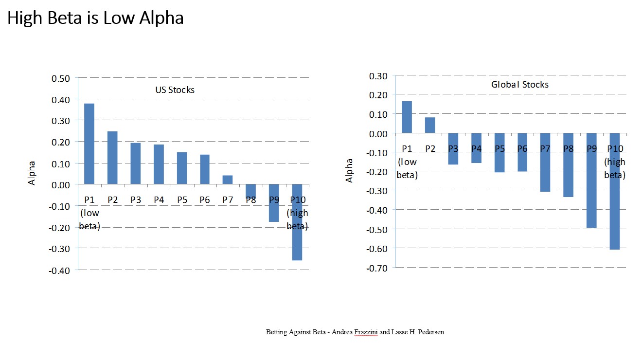
✅ This contradicts CAPM predictions and reveals an exploitable anomaly.
13.9.8.2.2. 2. Low Volatility Anomaly#
Source: Ang, Hodrick, Xing, Zhang (2006, 2009)
Stocks with lower total or idiosyncratic volatility have historically outperformed riskier stocks.
Intuition: Investors overpay for volatility (e.g., “lottery tickets”).
13.9.8.2.3. 3. Hedging Risk Factors#
Source: Hersovick, Moreira & Muir (2018)
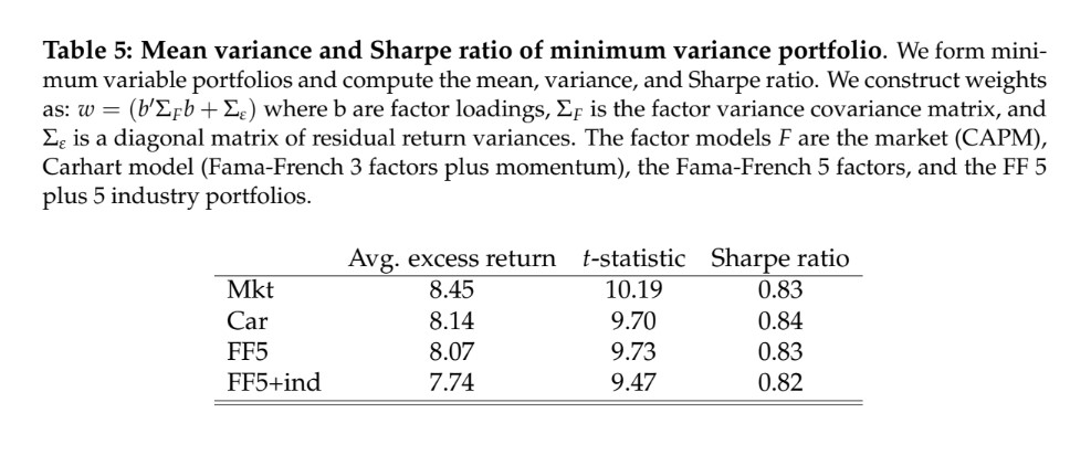
Rather than targeting individual stocks, this strategy builds minimum-variance portfolios relative to a factor model.
13.9.8.3. 🧮 How It Works (HMM Method)#
Choose a factor model:
Let ( F_t ) be a vector of factor returns (e.g., market, value, momentum, etc.).Run time-series regressions for each stock ( i ):
[ R^e_{i,t} = \alpha_i + \beta_{i,F} F_t + \varepsilon_{i,t} ]Build the total return covariance matrix:
Stack all ( \beta_{i,F} ) into a matrix
Assume residuals ( \varepsilon_{i,t} ) are uncorrelated across stocks (diagonal ( \text{Var}(\varepsilon) ))
Use: [ \text{Var}(R^e) = \beta \cdot \text{Var}(F_t) \cdot \beta^\top + \text{Var}(\varepsilon) ]
Construct the minimum variance portfolio: [ w \propto \text{Var}(R^e)^{-1} \cdot \mathbf{1} ]
This yields a zero-cost, risk-minimized portfolio that aggressively hedges exposure to systematic risk.
13.9.8.4. 📊 Empirical Results from HMM#
13.9.8.4.1. Portfolio Performance (Sharpe Ratios):#
13.9.8.4.2. Alpha Relative to Factor Models:#
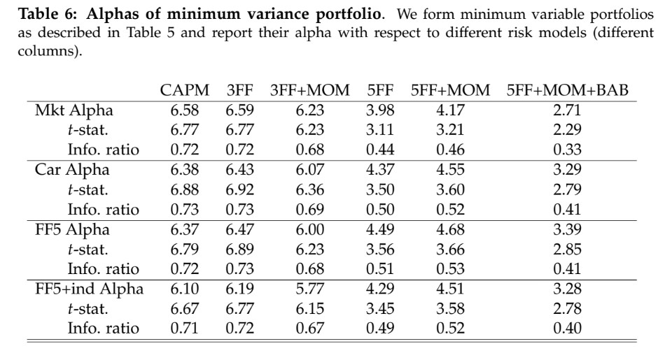
📌 These strategies deliver extremely high Sharpe ratios and alphas, consistently beating traditional models.
13.9.8.5. 🧠 Why Might This Work?#
Investors face leverage constraints: They prefer high-beta assets to boost returns, ignoring their poor risk-adjusted performance.
This creates overpricing in high-beta stocks and underpricing in low-beta stocks.
Defensive strategies exploit that mispricing, effectively betting against risk.
13.9.9. 🏆 Quality Investing#
What is “quality” investing?
It’s investing in businesses you’re willing to pay more for—all else equal. These firms are often fundamentally stronger: profitable, well-managed, and resilient.
13.9.9.1. 🔍 How Is Quality Defined?#
There’s no single definition, but common indicators include:
Profitability (gross profits, margins, ROE)
Safety (low leverage, stable earnings)
Good governance (shareholder-aligned incentives)
Growth (asset growth, earnings growth)
High payout ratios
Creditworthiness
Well-managed operations
Accounting quality (low accruals, consistent earnings)
In practice, many investors use composite quality scores that combine multiple of the above.
13.9.9.2. 🔁 Quality vs Value#
Value = Buy what’s cheap
Quality = Buy what’s strong
Yet the two are often linked:
“Buying high-quality firms without paying a premium is another form of value investing.”
💬 Warren Buffett:
“It’s far better to buy a wonderful business at a fair price than a fair business at a wonderful price.”
13.9.9.3. 💡 Simple Quality Signal: Gross Profitability#
One of the most effective and intuitive quality signals is:
[ \text{Gross Profitability} = \frac{\text{Revenue} - \text{COGS}}{\text{Assets}} ]
✅ Introduced in Novy-Marx (2013), this measure predicts returns even when controlling for book-to-market.
13.9.9.4. 📉 Why Might Quality Work?#
Rational view:
Productive firms (profitable) should command higher expected returns.
Investors might demand higher returns for riskier, lower-quality companies.
Behavioral view:
Investors overvalue “glamour” growth firms and neglect boring but profitable ones.
Mispricing arises when investors chase growth narratives without accounting for real productivity.
13.9.9.5. 🧪 Empirical Evidence#
Gross profitability strongly predicts returns—even after controlling for book-to-market.
Profitable firms:
Have higher average returns
Tend to have lower B/M ratios
Are larger (higher market caps)
📊 Evidence from Novy-Marx (2013):
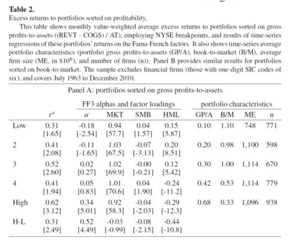
The Profitable Minus Unprofitable (PMU) portfolio earns a high alpha even relative to the Fama-French 3-factor model.
Fama and French later incorporated this into their 5-factor model as RMW (Robust Minus Weak).
The alpha is large in part because quality is negatively correlated with value—quality strategies tend to short cheap but low-quality stocks.
13.9.9.6. 🧩 Strategic Role of Quality#
Quality is a valuable hedge for value: it outperforms precisely when value underperforms.
Value strategies tend to hold low-quality names. Quality strategies often avoid them.
Combining value and quality enhances Sharpe and reduces downside risk.
📊 This synergy helps explain several other anomalies:
Return on Equity (ROE)
Net stock issuance
Default risk
Organizational capital
Earnings stability
Market power
13.9.9.7. 📈 Quality Expands the Frontier#
Quality doesn’t just earn returns—it helps explain others.
Robert Novy-Marx’s table shows that many previously “anomalous” strategies lose their alpha once the profitability factor is included:
📊 Impact of Profitability Factor:
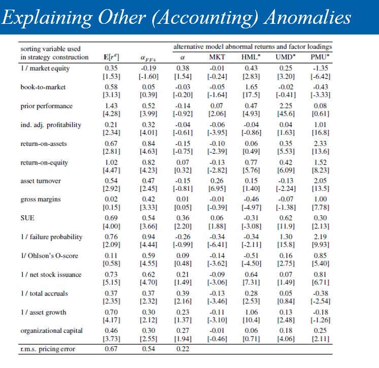
Columns 2 and 3 compare 4-factor vs 5-factor models.
Many alphas vanish when profitability is added—proving it spans the efficient frontier more effectively.