Introduction to Factor models

5. Introduction to Factor models#

🎯 Learning Objectives

By the end of this chapter, you should be able to:

Decode the α / β decomposition.
Learn how any asset’s excess return can be split into a factor‐driven piece (β × factor) and an asset-specific alpha, and see how this dual role lets factor models describe both risk and expected return.
Estimate factor exposure and alpha with regression.
Use time-series regressions of excess returns on factor returns to obtain β, α, residuals, and the associated statistics that guide portfolio design.
Create tracking and hedged portfolios.
Build a tracking portfolio equal to β times the factor, and a hedged (portable-alpha) portfolio that subtracts the tracking position—delivering pure alpha with zero in-sample factor risk.
Size positions under explicit risk budgets.
Apply volatility budgets at daily, monthly, or annual horizons; compute how much capital you can allocate to an unhedged position versus a hedged one, given its variance components.
Perform variance decomposition and risk-share analysis.
Break total variance into a factor part (β² Var f) and an idiosyncratic part (Var ε); measure the fraction of factor risk and adjust hedges to meet risk-share limits.
Build factor-implied covariance matrices.
See how a single-factor structure collapses the number of parameters from O(N²) to O(N); practice constructing the matrix as (B B’ Var f + \text{diag}(\sigma_ε^2)).
Appreciate the practical uses of factor models.
Understand why asset managers, pod shops, and risk desks rely on factor models to separate skill from beta, impose discipline on risk taking, and communicate performance.

5.1. Towards a factor Model#

First idea is that stocks might have different degree of co-movement
For example, Defensive stocks like utilities, supermarkets, and so on might not suffer as much when the market tanks
- Their cash flow might be more recession proof for example
- While luxury good producers like LMVH might be more sensitive to the stock market given its consumer base
Small stocks, stocks with high leverage and so one might particularly suffer during economic busts

\[(excess~return)=(intercept)+(stock~beta)*(factor~excess~return)+ (idio~risk)\]

fig, axes = plt.subplots(1, 2, figsize=(18,6))
import statsmodels.formula.api as smf


_temp= df_re.dropna(subset=['SPY', 'WMT'])

model = smf.ols(formula='WMT~SPY',data=_temp).fit()
intercept_wmt, beta_wmt = model.params
print(f'beta of asset WMT is {beta_wmt}')


axes[0].scatter(x=df_re['SPY'], y=(df_re['WMT']-beta_wmt*df_re['SPY']))
axes[0].set_title('SPY vs WMT Residuals')


_temp= df_re.dropna(subset=['SPY', 'JPM'])

model = smf.ols(formula='JPM~SPY',data=_temp).fit()
intercept_jpm, beta_jpm = model.params
print(f'beta of asset JPM is {beta_jpm}')


axes[1].scatter(x=df_re['SPY'], y=df_re['JPM']-beta_jpm*df_re['SPY'])
axes[1].set_title('SPY vs JPM Residuals')

plt.tight_layout()
plt.show()

beta of asset JPM is 0.6737719432407148
beta of asset JPM is 1.3949175281635984

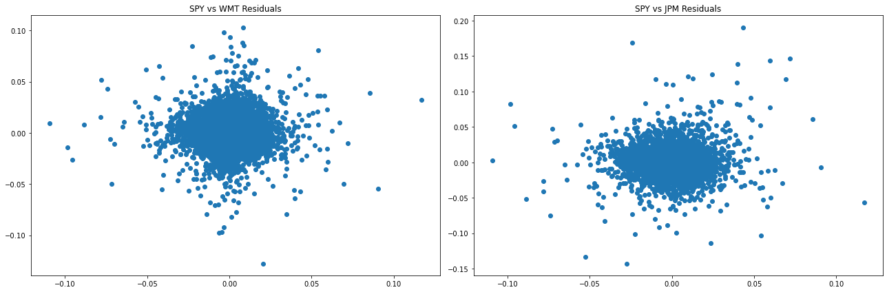
../../_images/fc368ce1918cc647735cdc1ad9893fb9f1df97a5fbe9e3c0870bc48c04473d7d.png

Did it work?

With the regression we have a statistical decomposition
At least in sample, the regression guarantees that the stock specific component is completely orthogonal to the factor

\[stock~specific~component=(excess~return)-(stock~beta)*(factor~excess~return)\]

df_re[['SPY']].corrwith(df_re['JPM']-beta_jpm*df_re['SPY'])

ticker
SPY    1.656269e-16
dtype: float64

df_re[['SPY']].corrwith(df_re['WMT']-beta_wmt*df_re['SPY'])

ticker
SPY    5.141267e-17
dtype: float64

How do we estimate the amount of idiosyncratic risk?

How do we estimate the amount of systematic risk?

5.2. Factor Models come in two flavors#

It can be useful for measuring risk if
- The risk $\epsilon$ is specific to asset $i$ and only weakly correlated with other assets (ideally completely)
- i.e if the factor explains lots of the common variation in stock returns
- You don’t really care whether the factors face premia, but only if they explain variation in returns
It can be useful for measuring expected returns if
- The premium on the factor f, $E[f]$ summarize well the known “priced” systematic risk factors
- By “priced” we mean risk-factors that earn a risk premium $E[f]>0$
- A model can be a good model of expected returns, but not explain much of realized returns
- Such model is useful for performance evaluation

We will call the first a factor model of risk, and the second a factor model of expected returns. However, this distinction is often blurry. Arbitrage logic tells us that if we have a really good model of risk, we should also have a good model of expected returns But in practice for stocks, there is lots and lots of unexplained variation

People start with a factor model with priced factors and then add additional factors to explain risk.

Let $r^e$ be an asset excess return over the risk-free rate

Let $f$ be a traded factor, for now the excess returns on SPY ETF (that holds a basket that replicates the S&P 500 index)

Then we can write

\[r^e=\alpha + b*f+\epsilon\]

where $b$ is asset $i$ exposure to the factor $f$

We can always write things that way–it is just a statistical decomposition

Whether we are working with a “Risk Model” or an “Expected Return” model will come down to the following

For risk model we assume $\epsilon$ uncorrelated across stocks
For Expected return model, we assume $\alpha=0$ for all stocks/strategies

What use is a factor model?

the alpha/Beta decomposition is how the money management industry is organized.
- Big pay days only if people think you have alpha
- Getting exposure to the factor is a commodity. Anyone can buy SPY or many other funds that track the market very well
- In most funds, specially for portfolio managers working a pod shops like Citadel (https://www.wsj.com/finance/investing/citadel-ken-griffin-hedge-funds-c9ddf51d) and Millenium (https://www.wsj.com/finance/investing/the-giant-hedge-fund-that-hates-risk-and-still-wins-1110e90a), a portfolio manager mandate is to take no factor risk–or at least aim to be close to factor neutral.
- It is all about the alpha
factor models allow you to understand and hedge risk
- This is essential if you want to concentrate your portfolio only on risks that you get compensated for holding

5.3. Alpha and Beta(s)#

Note that

\[E[r]=E[rf+r^{e}]=rf+E[\alpha_i + b*f+\epsilon]\]

\[E[r]=rf+\alpha+b*E[f]+E[\epsilon]\]

Using that $E[\epsilon]=0$ we have $$E[r]=rf+\alpha+b*E[f]$$
Thus, just like the risk of our asset could be attributed to the factor and it’s component, the same model also allow us to decompose the expected return in terms of the risk-free rate, the premium coming from the common factor exposure $b*E[f]$ and the risk-premium specific to the asset, the ALPHA.
The alpha does not need to be in a specific asset, can be o a combination of them
The decomposition works the same for portfolio of assets
For now we have a single factor, but you will see that as you have more factors, everything is pretty much the same

5.4. Focus on your skill, hedge all the residual risk#

No matter who you are, you will face dollar risk limits

So it is essential that you deploy risk wisely

The key use of the factor model is to give you discipline to separate your edge from the rest

How to use the factor model?

First , realize that each piece of the factor model will require very thoughtful estimation

Even here with only one asset and one factor we already need to know many things

The risk-free rate
The strategy/asset factor beta
The factor risk-premia
The factor variance
The strategy/asset specific alpha
The strategy/asset specific variance

For now we will assume we know each of these.

if you have an asset that has alpha, says, you are confident that APPLE will beat expectations and you expect a 5% appreciation in the next 12 months beyond any factor exposure that Apple might had, what do you do?

Buy apple!

But what if the market crashes? Why bear that risk?
Portfolio allocators look for managers with alpha, not beta. What if the market crashes before apple surprises and your investors pull out?

Hedge the market
- How do you do that?
- Short it!
- How much?
- the strategy beta!

Example:

You buy 1M in Apple stock, so your portfolio PnL is 1M*$r^{apple}$
Your portfolio PnL in excess what you would earn in treasuries is 1M*$(r^{apple}-rf)$
Sell (short) 1M*$beta_{apple,f}$ of the factor
Now your portfolio PnL above the risk-free rate is

\[1M*(r^{apple}-rf-\beta*r^{SPY}+\beta*rf)\]

When you sell SPY short you get the money and here I am “investing” it in the risk-free rate

Alternatively you can think of it as using to fund the apple buy

it does not matter, because we are accounting for the time-value of money

We certainly don’t want to invest any other risk assets as it would just add noise to our trade

\[1M*(r^{apple}-\beta*r^{SPY}-(1-\beta)*rf)\]

For a high beta stock your trade generates extra cash!

If $\beta>1$, $-(1-\beta)*rf>0$

This happens because you are selling more than you are buying

If we substitute our factor model in our trade PnL and take expectations what do we get?

\[1M*E[r^{apple}-rf-\beta*r^{SPY}+\beta*rf)]\]

\[1M*E[\alpha_i+rf+beta*(r^{SPY}-rf)+u_i-rf-\beta*r^{SPY}+\beta*rf)]\]

A pure play portfolio!

\[1M*E[\alpha_i]\]

And what is the portfolio risk?

\[std(1M*(r^{apple}-rf-\beta*r^{SPY}+\beta*rf))=1M*std(u_i)\]

We refer to portfolio $(1,-\beta)\times(AAPL,SPY)$ as the Apple-factor hedged portfolio, or simply the “hedged-portfolio”
and refer to $-\beta \times $ (SPY) as the “Hedging Portfolio”

Implementing

Lets do this!

I will use a regression to get some numbers for us to do this strategy

but for now, just think those as numbers I am giving you and don’t think of the regression as giving the right numbers necessarily.

%pip install wrds
import wrds

conn = wrds.Connection()
ticker=['MSFT']
df_returns = get_daily_wrds(conn,tickers=ticker)
print(df_returns.head())
df_returns.describe()

WRDS recommends setting up a .pgpass file.
Created .pgpass file successfully.
You can create this file yourself at any time with the create_pgpass_file() function.
Loading library list...
Done
[10107]
ticker          MSFT
date                
1986-03-14  0.035714
1986-03-17  0.017241
1986-03-18 -0.025424
1986-03-19 -0.017391
1986-03-20 -0.026549

ticker	MSFT
count	9778.000000
mean	0.001128
std	0.021017
min	-0.301158
25%	-0.009079
50%	0.000380
75%	0.011193
max	0.195652

df_factor = get_factors()
print(df_factor.head())
df_factor.describe()

                 RF  Mkt-RF
Date                       
1963-07-01  0.00012 -0.0067
1963-07-02  0.00012  0.0079
1963-07-03  0.00012  0.0063
1963-07-05  0.00012  0.0040
1963-07-08  0.00012 -0.0063

	RF	Mkt-RF
count	15481.000000	15481.000000
mean	0.000173	0.000281
std	0.000125	0.010196
min	0.000000	-0.174400
25%	0.000070	-0.004200
50%	0.000180	0.000500
75%	0.000240	0.005100
max	0.000610	0.113500

# I will align the two dataframes to ensure that the dates are the same

df_return, df_factor = df_returns.align(df_factor, join='left', axis=0)

df_eret=df_return['MSFT']-df_factor['RF']
import statsmodels.api as sm

X = df_factor['Mkt-RF']
X = sm.add_constant(X)  # Adds a constant term to the predictor
y = df_eret

model = sm.OLS(y, X).fit()
print(model.summary())

                            OLS Regression Results                            
==============================================================================
Dep. Variable:                      y   R-squared:                       0.415
Model:                            OLS   Adj. R-squared:                  0.415
Method:                 Least Squares   F-statistic:                     6937.
Date:                Mon, 24 Mar 2025   Prob (F-statistic):               0.00
Time:                        13:47:17   Log-Likelihood:                 26515.
No. Observations:                9778   AIC:                        -5.303e+04
Df Residuals:                    9776   BIC:                        -5.301e+04
Df Model:                           1                                         
Covariance Type:            nonrobust                                         
==============================================================================
                 coef    std err          t      P>|t|      [0.025      0.975]
------------------------------------------------------------------------------
const          0.0006      0.000      3.601      0.000       0.000       0.001
x1             1.1872      0.014     83.288      0.000       1.159       1.215
==============================================================================
Omnibus:                     1451.257   Durbin-Watson:                   1.929
Prob(Omnibus):                  0.000   Jarque-Bera (JB):            22136.865
Skew:                           0.141   Prob(JB):                         0.00
Kurtosis:                      10.366   Cond. No.                         87.7
==============================================================================

Notes:
[1] Standard Errors assume that the covariance matrix of the errors is correctly specified.

alpha=model.params[0]
beta=model.params[1]
var_r=y.var()
var_f=df_factor['Mkt-RF'].var()
var_e=model.resid.var()
mu_f=df_factor['Mkt-RF'].mean()
print(f"Alpha: {alpha}")
print(f"Beta: {beta}")
print(f"Variance of MSFT returns (var_r): {var_r}")
print(f"Variance of market factor (var_f): {var_f}")
print(f"Variance of residuals (var_e): {var_e}")
print(f"Mean of market factor (mu_f): {mu_f}")

Alpha: 0.0005855699261548292
Beta: 1.187234068887255
Variance of MSFT returns (var_r): 0.0004416123295030902
Variance of market factor (var_f): 0.00013005387619649368
Variance of residuals (var_e): 0.00025831692182161234
Mean of market factor (mu_f): 0.00035668848435262666

Stop and Think

What frequency are these parameters?

How to I make it comparable say with the annual risk-free rate?

What does the alpha mean? How should you think about it? Do you think is informative about future MSFT alpha? Why? Why not?

What about the variance terms? And the covariance terms?

5.5. Tacking, Hedging and Hedged portfolios#

Tracking Portfolios

We also refer to it as “hedging portfolios” or “mimicking portfolios”

Tracking portfolios are the portfolios that use a set of factors to track the returns on an asset.

It can be used as a way to construct hedges for corporations, hedges for trading strategies, or a way to define a benchmark for an active management.
It is used to construct what people in the industry calls “portable alpha”, because it allows one to separate the alpha of a trading strategy’s factor exposure
The idea of the tracking portfolio is to track the component of an asset return that can be obtained by investing in a simple traded factor (or combos of traded factors). For now, this means the market portfolio.
For a given factor model representation of a trading strategy

\[r^e_i=\alpha_i+\beta_if+\epsilon_i, \]

with $var(\epsilon_i)=\sigma_e^2$
the $i^{th}$ Tracking portfolio is $\beta_iW^{MKT}$, where $W^{MKT}$ is the vector of weights of the market portfolio.
or if one is trading directly on the total market portfolio as an asset, the tracking portfolio weight on the market portfolio asset is simply $\beta_i$

In our case above we say the tracking portfolio of the stock is $\beta$ and the hedging portfolio -$\beta$ on the market

# Returns on the tracking portfolio

Portfolio=df_eret
MKT=df_factor['Mkt-RF']
Tracking=MKT*beta

plt.scatter(x=Portfolio,y=Portfolio)
plt.scatter(x=Portfolio,y=Tracking)
plt.show()

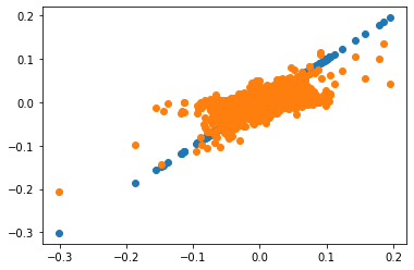
../../_images/a31fcc2d4636bbcedc7e286e030f9e6f928d2663aae7d5d8ddd3678630011bb7.png

We see here the obvious fact that we cannot track at all variation in the market with the market portfolio so they capture different risks
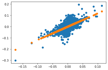
Another way of looking at it is to put the factor returns on the x-axis
The tracking is a perfect straight line where the slope is the beta of the asset

Portfolio=df_eret
MKT=df_factor['Mkt-RF']
Tracking=MKT*beta

plt.scatter(x=MKT,y=Portfolio)
plt.scatter(x=MKT,y=Tracking)
plt.show()

../../_images/529c85e27d1c0976bbbf7df032c759324d693aae39f953ee1ebd71b5fca915d1.png

Hedged portfolio

The Hedged strategy return (also called portable alpha) is

\[r^{hedged}_i=r^e_i-\beta_ir^{MKT}\]

This portfolio can be constructed simply by $W^i-\beta^iW^{MKT}$, the weights of the trading strategy minus the tracking portfolio weights.
The excess returns take out risk-free rate effects, and the hedged portfolio takes out market factor effects

A few observations

The mean return of the hedged portfolio is just the time series alpha!
The volatility of the strategy is the vol of the residuals of the time series regression
If you run a regression on the market you will see that the hedged portfolios have $\beta=0$, which is by construction.
This is the reason why sometimes people call these portfolios “Pure Alpha”, or as Bridgwater calls it, “Portable Alpha”

# Returns on the hedged portfolio
Hedged=Portfolio-Tracking

plt.scatter(x=MKT,y=MKT)
plt.scatter(x=MKT,y=Hedged)
plt.show()

../../_images/fd2e14200957ae30c823a81e42f72cd6cad0c658ee685fff86c01f37a7424e3d.png

Insight

The average excess return on the hedged portfolio is the alpha of the unhedged portfolio! Intuition: The hedged portfolio has mechanically zero beta (in-sample) so it’s excess return is “pure” alpha

print('hedge portfolio excess returns')
print(Hedged.mean()*12)
print('alpha of unhedge portfolio')
print(alpha*12)

hedge portfolio excess returns
0.007026839113857923
alpha of unhedge portfolio
0.007026839113857951

Factor Models and Risk Budgets

Lets say we have 1 million dollar per month volatility (i.e. standard deviation) budget

What that means?

Means that the size of my position times the monthly volatility of my position must be less than 1 million dollars?

Why you might impose such a cap?

How much o MSFT can I own?

If I invest one dollar in MSFT I get: $1*\sqrt(var_r*252)$ standard deviation for 1 year
If I invest one dollar in MSFT I get: $1*\sqrt(var_r*21)$ standard deviation for 1 month

To get 1M per month I invest $\frac{1M}{\sqrt(var_r*21)}$

x=1/(var_r*21)**0.5
x

10.384121419128503

What does that mean? How many million dollars I can buy of the stock?

What if the budget was for 1 year? How many would I be able to buy?

What is your expected PnL in the end of the year?
- Here we will subtract you funding costs, which I will assume is also rf so it will be a wash

\[x*(rf+\beta*\mu_f+\alpha-rf)*252\]

What is your Expected PnL after your market exposure is subtracted

\[x*(\alpha)*252\]

print(x*(beta*mu_f+alpha)*252)
print(x*(alpha)*252)

0.7686879316063537
0.4596563249799126

Often shops have risk-adjusted PnL. So while you might expect to make x*(beta*mu_f+alpha)*252 for the fund, they only comp you based on x*(alpha)*252

Focusing on your edge

Now suppose you focus your edge–i.e. investing in MSFT but hedging the market risk

How much of the market do I need to short per dollar invested in MSFT?

you short exactly it’s beta

\[x_h=-\beta\]

So your portfolio is

\[x*(stock:1,market:-\beta)\]

How many dollars in MSFT can I buy? (lets say for a yearly budget)

\[\frac{1M}{\sqrt(var_e*252)}\]

xe=1/(var_e*252)**0.5
xe

3.8831665045807324

Why $var_e$ is the volatility of the hedge portfolio?

Note that the hedged portfolio return is

\[rh=re-\beta*f=\alpha+\epsilon\]

Note that $E[f\epsilon]=0$ as beta is such that there is no factor risk left in the residuals ( that is the OLS regression assumption!)

The leftover risk is exactly orthogonal to the factor risk

This what makes this the optimal hedge portfolio–> it hedges all the market risk!

So it follows that

\[Var(rh)=Var(\alpha+\epsilon)=Var(\epsilon)\]

What is you expected PnL?
What is you expected “factor-adjusted PnL”?

xe*(alpha*252)

0.6005130298526444

What is your portfolio Sharpe Ratio? what is Sharpe Ratio anyways?
What is you portfolio Sharpe with the hedge and without the hedge?

5.6. Variance Decomposition#

Factor models are essential to manage risk

A pod shop manager , a manager in a mutual fund in a large mutual fund company, a hedge fund trader in a large hedge fund,…all of those will typically have tight limits on the TOTAL risk of their portfolio, i.e. $var(r)$ but also on the factor component of their portfolio

But even if you don’t, and you are an active manager with freedom of trading, you still want to control quite carefully how much non-essential risks you are taking in your portfolio

The decomposition here with single factor is really easy, but once you understand it, the multi-factor decomposition will be also easy to understand ( even it a little more involved)

The total variance of your strategy/asset is

\[Var(r^e)=Var(\alpha +b*f+\epsilon)=Var(b*f)+Var(\epsilon)=b^2Var(f)+var(\epsilon)\]

We can see already the factor part $(b^2Var(f))$ and the idiosyncratic part $var(\epsilon)$. It decomposes nicely because e and f are orthogonal.

The fraction of factor risk in your portfolio is

\[\frac{b^2Var(f)}{Var(r^e)}\]

You factor risk depends

on your factor beta–this might grow in a market turmoil for example
on the factor variance–also might grow when markets are choppy

The factor risk-share also depend on the idio vol. During a market turmoil all vols tend to go up, but factor vols tend to go up more So both your total risk grows as the share of factor risk

beta**2*var_f/var_r

0.4141025460425463

Suppose I want to get this to the 20% limit. What do I do?

Lets say xh is your position on the market, then your portfolio is

\[rp=x(1*re+xh*f)\]

You want the factor piece to be less than vbar=20%

\[Var(rp)=Var(x(1*re+xh*f))=Var(x(1*(\alpha+\beta*f+\epsilon)+xh*f))=Var(x(\beta+xh)*f)+x^2Var(\epsilon)\]

\[Var(rp)=x^2(\beta+xh)^2*Var(f)+x^2Var(\epsilon)\]

so we need

\[\frac{x^2(\beta+xh)^2*Var(f)}{x^2(\beta+xh)^2*Var(f)+x^2Var(\epsilon)}=vbar\]

Note that your size of your overall portfolio cancels out.

What matters for the share is your hedge per unit of position

\[\frac{(\beta+xh)^2*Var(f)}{(\beta+xh)^2*Var(f)+Var(\epsilon)}=vbar\]

reorganizing

\[(\beta+xh)^2*Var(f)=vbar*((\beta+xh)^2*Var(f)+Var(\epsilon))\]

\[(1-vbar)(\beta+xh)^2*Var(f)=vbar*Var(\epsilon)\]

\[(\beta+xh)^2=\frac{vbar*Var(\epsilon)}{(1-vbar)Var(f)}\]

\[(\beta+xh)=\sqrt{vbar\frac{Var(\epsilon)}{(1-vbar)Var(f)}}\]

\[xh=\sqrt{\frac{vbar*Var(\epsilon)}{(1-vbar)Var(f)}}-\beta\]

What is the hedge portfolio if you want zero factor risk?

vbar=0.2
xh20=((vbar*var_e)/((1-vbar)*var_f))**0.5-beta
xh20

-0.4816910986685352

5.7. Factor models and Variance-covariance Matrixes Estimation#

We will see how we can compute covariance matrixes easily under the assumption that the factor captures most sources of co-movement across stocks

In this case the assumption is very bad…and not even close to holding for most assets…but will allow us to get the intuition

We will then learn how to do it with many factors as is standard in the industry

Here I will use i,j for a individual stock

\[r^{e,i}=\alpha_i+\beta_{i,f}f+\epsilon_{i}\]

non-factor component $\epsilon_i$ of the asset return of asset $i$. Assumed to uncorrelated between any two assets

Now this is just a regression!

We have that

\[Var(r^{e,i})=\beta_i^2Var(f)+var(\epsilon_{i})\]

This gives us a nice decomposition of risk as we saw above

the risk component that is driven by the common factor
the asset specific comment

Now if our assumption holds,i.e. the non-factor risk is uncorrelated across assets

\[cov(\epsilon_{i,t},\epsilon_{j,t})=0\]

This will never hold in any sample. It is an assumption that you impose after you think that you add enough factors to capture the co-movement across assets

Then

\[Cov(r_t^{e,i},r_t^{e,j})=Cov(\alpha_i+\beta_{i}f_t+\epsilon_{i,t},\alpha_j+\beta_{j}f_t+\epsilon_{j,t})=\beta_i\beta_jVar(f_t)\]

And the covariance matrix is simply

\[\begin{split} \left[\begin{array}{cc} \beta_i^2 & \beta_i\beta_j \\ \beta_i\beta_j & \beta_j^2 \end{array}\right]var(f_t)+\left[\begin{array}{cc} var(\epsilon_{i,t}) & 0 \\ 0& var(\epsilon_{j,t}) \end{array}\right]\end{split}\]

We see that now for N assets we only need to estimate N factor exposures, N asset specific volatilities , and the factor volatility

If we were estimating a variance-covariance matrix without imposing the factor model we would have to estimate N covariances and $(N^2-N)/2$ covariance terms: $2N+1$ vs $(N^2-N)/2+N$ is huge as N grows

Practice

Choose a five tickers you like plus SPY

Estimate their unrestricted covariance matrix

Estimate the single-factor model (single factor=SPY)

Build the factor implied covariance matrix

Can you compare the number of parameters you need to estimate in each case

Can you discuss if it such model is a good one in this case

📝 Key Takeaways

Factor models separate what you earn from what you ride.
Beta captures common market movements; alpha is the slice of return not explained by those movements.
Hedging out β turns views into “portable” alpha.
Going long the asset and short β units of the factor neutralizes systematic risk, leaving a position whose mean excess return equals its alpha and whose volatility equals the residual variance.
Risk budgets shrink once you hedge intelligently.
A hedged position’s lower volatility allows you to deploy more capital for the same risk cap—and to earn more alpha-attributed P&L.
Variance decomposition is your monitoring dashboard.
It tells you how much of today’s risk is coming from factors versus idiosyncratic shocks and highlights when market turmoil swells the factor share.
Tracking portfolios clarify performance attribution.
By explicitly matching the factor component, you can assess whether a manager’s outperformance is genuine skill or just hidden beta.
Factor-implied covariance matrices are parsimonious and , maybe, more intuitive.
Estimating only N betas, N idiosyncratic variances, and one factor variance yields a workable covariance estimate even when the full N × N matrix is unmanageable.
All numbers are frequency-specific.
Alpha, variances, co-variances and Sharpe ratios must be annualized (or otherwise scaled) consistently before comparison or budgeting. Beta is the only one that is theoretically invariant
Good questions drive good models.
Throughout the notebook “Stop and Think” prompts remind you to check data frequency, interpret α’s forecasting value, and judge whether the single-factor assumption is adequate for your application.