
10.1. Expected Return Timing#
The most classic timing strategies are motivated by the fact that high dividend yield periods seems to be followed by above average returns
The plot shows the dividend-yield of the stock market overlayed with the future 7 year returns
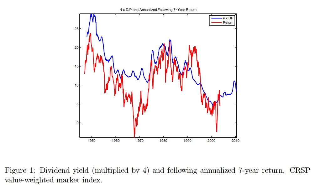
It tell us that in this sample, periods when the dividend yield was high were periods where the returns were really high going forward.
This might be intuitive to you, but it is really a fact that puzzled lots of people and earned Robert Shiller a nobel prize

It tells us that when the price (per dividend) is low what actually happens is NOT that the dividends go down going forward which would be intuitive–if the price is low is probably because payouts will be low– but instead prices go up–meaning expected returns were high!
So this suggests EXPECTED returns to invest in the market change a lot overtime.
A trading strategy that exploits this would have weights that depend on the dividend yield signal.
#!pip install wrds
# import wrds
db = wrds.Connection()
crsp_sql = f"""
    SELECT date, vwretd, vwretx
    FROM crsp.msi
    ORDER BY date;
"""
crsp = db.raw_sql(crsp_sql, date_cols=['date'])
crsp['dp'] = (1.0 + crsp['vwretd']) / (1.0 + crsp['vwretx']) - 1.0
crsp = crsp.set_index('date')
crsp
WRDS recommends setting up a .pgpass file.
Created .pgpass file successfully.
You can create this file yourself at any time with the create_pgpass_file() function.
Loading library list...
Done
| vwretd | vwretx | dp | |
|---|---|---|---|
| date | |||
| 1925-12-31 | NaN | NaN | NaN |
| 1926-01-30 | 0.000561 | -0.001395 | 0.001959 |
| 1926-02-27 | -0.033046 | -0.036587 | 0.003675 |
| 1926-03-31 | -0.064002 | -0.070021 | 0.006472 |
| 1926-04-30 | 0.037029 | 0.034043 | 0.002888 |
| ... | ... | ... | ... |
| 2024-08-30 | 0.021572 | 0.020203 | 0.001342 |
| 2024-09-30 | 0.020969 | 0.019485 | 0.001456 |
| 2024-10-31 | -0.008298 | -0.009139 | 0.000849 |
| 2024-11-29 | 0.064855 | 0.063463 | 0.001309 |
| 2024-12-31 | -0.031582 | -0.033470 | 0.001953 |
1189 rows × 3 columns
# we will average over 1 year to get rid of seasonality and noise in general
# we will also multiply by 12 to get the annualized dividend yield
(crsp.dp.rolling(window=12).mean()*12).plot()
<Axes: xlabel='date'>
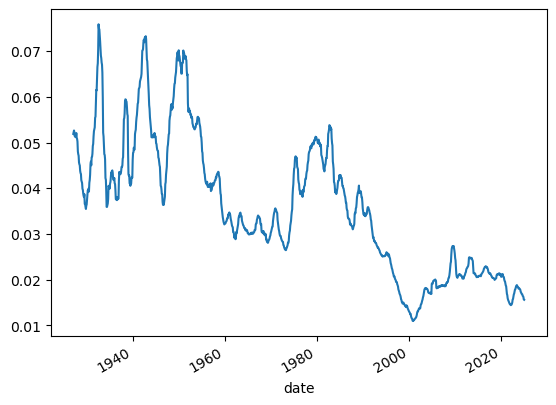
dividend yields went from 4%-7% in the start of the sample (1930’s) to around 2% now
We will now look at the relationship between dividend yields and 5-year ahead returns
That is, I will ask the regression to tell me: if I see a high dividend-yield what does typically happen with the returns of my investment in the market if I buy it and hold it for 5 years
Because this story is mostly about risk-premia we will take out the risk-free rate
df = get_factors('CAPM', freq='monthly').dropna()

# We align the indices of the CRSP data and the Fama-French data
# they are both monthly data but wrds has the actual last trading date of the month while
# the Fama-French data has the last calendar day of the month

crsp.index = crsp.index+pd.offsets.MonthEnd(0)
years=5
merged_data = crsp.merge(df[['RF']], left_index=True, right_index=True)
# here we cumulate the excess returns over the next 5 years
# we do that by first taking a rolling product of gross returns--the windown is backwards looking
# then we shift the result by 5 years to get the future returns
merged_data['R_future']= (1+merged_data['vwretd']-merged_data['RF']).rolling(window=years*12).apply(np.prod).shift(-years*12)**(1/years)-1
# I averaging the dividend yield to get rid of seasonality and noise
# a simiar possibility would be to add the dividends for the last 12 months and divide by the price at the end of the period
# I am multiplying by 12 to get the annualized dividend yield
merged_data['dp_avg'] = merged_data.dp.rolling(window=12).mean()*12
#finally I multiply the dividend yield by 3 to make it more visible in the plot
ax=(merged_data['dp_avg']*3).plot()
merged_data[['R_future']].plot(ax=ax)
c:\Users\alan.moreira\Anaconda3\lib\site-packages\pandas_datareader\famafrench.py:114: FutureWarning: The argument 'date_parser' is deprecated and will be removed in a future version. Please use 'date_format' instead, or read your data in as 'object' dtype and then call 'to_datetime'.
  df = read_csv(StringIO("Date" + src[start:]), **params)
<Axes: >
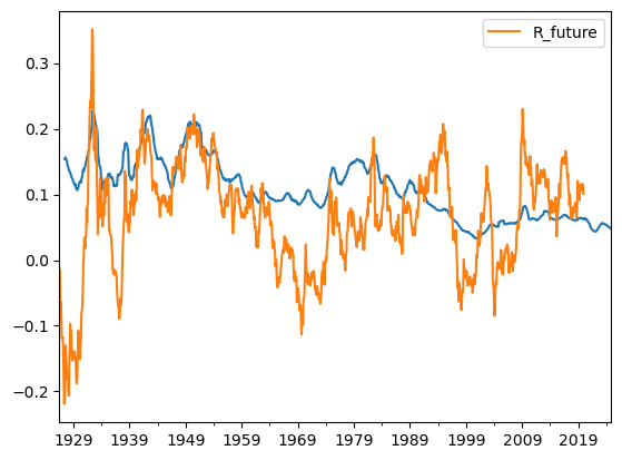
#raw correlation suggests interesting relationship
# this is predictive
(merged_data['dp_avg']).corr(merged_data['R_future'])
0.3670940450303395
How do you see if the signal works?
You start with some signal that you know in date \(t\)
Estimate the forecasting regression
The difference from factor models is that the relationship is NOT contemporaneous
The whole point is to use the fact that you know the signal ahead of time
That is the signal at date \(t\) has information about the return in data \(t+1\) (or some longer horizon)
In fact what we will do below is to try to predict the next 5 years
We will be looking at the b coefficient, it’s standard errors and the r-squared of this regression
Is the R-squared meaningful ( we will discuss later ) and the b is well estimate and different from zero?
If the answer is no: STOP, the signal does not work even in sample!
If yes, then you kick the tires more…
# lets run the regression
import statsmodels.api as sm
X = sm.add_constant(merged_data['dp_avg'] )
model = sm.OLS(merged_data['R_future'], X, missing='drop').fit()
print(model.summary())
                            OLS Regression Results
==============================================================================
Dep. Variable:               R_future   R-squared:                       0.127
Model:                            OLS   Adj. R-squared:                  0.127
Method:                 Least Squares   F-statistic:                     161.8
Date:                Thu, 14 Aug 2025   Prob (F-statistic):           1.08e-34
Time:                        16:47:16   Log-Likelihood:                 1299.2
No. Observations:                1111   AIC:                            -2594.
Df Residuals:                    1109   BIC:                            -2584.
Df Model:                           1
Covariance Type:            nonrobust
==============================================================================
                 coef    std err          t      P>|t|      [0.025      0.975]
------------------------------------------------------------------------------
const          0.0297      0.006      4.878      0.000       0.018       0.042
dp_avg         1.9598      0.154     12.719      0.000       1.657       2.262
==============================================================================
Omnibus:                      234.961   Durbin-Watson:                   0.044
Prob(Omnibus):                  0.000   Jarque-Bera (JB):              563.442
Skew:                          -1.134   Prob(JB):                    4.47e-123
Kurtosis:                       5.651   Cond. No.                         68.4
==============================================================================

Notes:
[1] Standard Errors assume that the covariance matrix of the errors is correctly specified.
WOW! Look at this t-stat!
What do you think? Can we really take it to the bank?
The summary is
This regression has many issues and academics have spent a lot of time on it
There is a relationship but it is weak
You absolutely cannot take it to the bank
The big issues are:
the variable dividend yield is extremely persistent, so we do not have that much variation in it. Just a few data points even in a long sample
The return are overlapping, so when we cumulate the returns we are really double counting the number of observations, so the traditional standard errors are totally off
Traditional–but not bullet proof is to use an adjusted standard errors like HAC with a window consistent with the rolling window. We do that below and does make a huge difference
The third issue is that there is a bias in the regression because the innovation in the variables are correlated
import statsmodels.api as sm
X = sm.add_constant(merged_data['dp_avg'] )
model = sm.OLS(merged_data['R_future'], X, missing='drop').fit(cov_type='HAC', cov_kwds={'maxlags': years*12})
print(model.summary())
                            OLS Regression Results
==============================================================================
Dep. Variable:               R_future   R-squared:                       0.127
Model:                            OLS   Adj. R-squared:                  0.127
Method:                 Least Squares   F-statistic:                     11.89
Date:                Thu, 14 Aug 2025   Prob (F-statistic):           0.000584
Time:                        14:45:06   Log-Likelihood:                 1299.2
No. Observations:                1111   AIC:                            -2594.
Df Residuals:                    1109   BIC:                            -2584.
Df Model:                           1
Covariance Type:                  HAC
==============================================================================
                 coef    std err          z      P>|z|      [0.025      0.975]
------------------------------------------------------------------------------
const          0.0297      0.024      1.232      0.218      -0.018       0.077
dp            23.5177      6.819      3.449      0.001      10.153      36.883
==============================================================================
Omnibus:                      234.961   Durbin-Watson:                   0.044
Prob(Omnibus):                  0.000   Jarque-Bera (JB):              563.442
Skew:                          -1.134   Prob(JB):                    4.47e-123
Kurtosis:                       5.651   Cond. No.                         819.
==============================================================================

Notes:
[1] Standard Errors are heteroscedasticity and autocorrelation robust (HAC) using 60 lags and without small sample correction
one thing that people do to evaluate these forecasting regressions is loot at the R-squared out of sample relative to some benchmark \(\mu_{t}\).
A less “academicy” way is to simply see how well the trading strategy does out of sample
How would we do that?
for example you would have a weight
where a b are the regression coefficient on the market excess return, and \(a+b\frac{d_t}{p_t}\) is our premium forecast
\(\gamma\) is the risk-aversion and \(\sigma\) is the volatility of the asset.
So your strategy return is
Where you would use to control your average exposure to the market.
Or more simply
If x<1, invest in the risk-free rate, if x>1, borrow to fund a bigger position in the risky asset
Estimation_sample=merged_data[:'2005'].copy()
Test_sample=merged_data['2006':].copy()
years=5
Estimation_sample['R_future']= (1+Estimation_sample['vwretd']).rolling(window=years*12).apply(np.prod).shift(-years*12)**(1/years)-1

X = sm.add_constant(Estimation_sample['dp_avg'] )
model = sm.OLS(Estimation_sample['R_future'], X, missing='drop').fit(cov_type='HAC', cov_kwds={'maxlags': years*12})


gamma=2
vol=0.16

Test_sample['premium_forecast']=(model.params['const']+model.params['dp_avg']*Test_sample['dp_avg'])
Test_sample['weight']=Test_sample['premium_forecast']/(gamma*vol**2)

Test_sample['weight'].plot()
<Axes: >
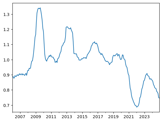
Note that the denominator here \(\gamma \sigma^2\) is only impacting your average position in the asset
An alternative it to pick it so that you have some average desired position in the asset
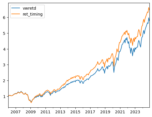
We can now directly look at it’s performance relative to a buy and hold strategy
Test_sample['ret_timing']=Test_sample['RF']+Test_sample['weight']*(Test_sample['vwretd']-Test_sample['RF'])

(1+Test_sample[['vwretd','ret_timing']]).cumprod().plot()
<Axes: >
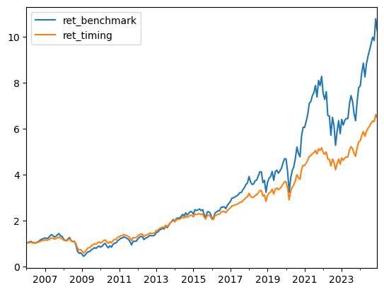
But is this the right benchmark for performance?
Here is a different one
Here we use the average return in the estimation sample as our measure of risk-premium
premium_benchmark=(Estimation_sample['vwretd']-Estimation_sample['RF']).mean()*12
Test_sample['weight_benchmark']=premium_benchmark/(gamma*vol**2)
Test_sample['ret_benchmark']=Test_sample['RF']+Test_sample['weight_benchmark']*(Test_sample['vwretd']-Test_sample['RF'])
(1+Test_sample[['ret_benchmark','ret_timing']]).cumprod().plot()
<Axes: >
Does it work or not?
How to evaluate?
if you are interested in digging further see
John Y. Campbell, Samuel B. Thompson, Predicting Excess Stock Returns Out of Sample: Can Anything Beat the Historical Average?, The Review of Financial Studies, Volume 21, Issue 4, July 2008, Pages 1509–1531, https://doi.org/10.1093/rfs/hhm055
We refer to the dividend-yield as a signal
There are many other signals that have been show to predict market returns– in the past
Harder to know which ones work right now
Some of the signals are
Short interest (The size of short positions relative to the overall market)
idea: shorts must know what they are doing and if the short is high things will be bad
Variance risk premium (VIX-squared-Realized Variance)
If risk-premium in option markets is high, risk premium in equity markets is probably high
Equity issuing activity (fraction of the market being sold)
If companies are issuing a lot they must think they are overvalued
Aggregate accruals
I think the idea here is that accruals capture manipulation so if firms are doing a lot of of it, it might mean that bad news are about to land and returns will be low going forward