
4. Introduction to Asset Returns#
🎯 Learning Objectives
By the end of this chapter, you should be able to:
Define and compute total returns
Build returns from price and dividend data, recognizing that “return” is the normalized gain relative to the initial price and works for any positive‐priced asset.Strip out the risk-free rate
Convert raw returns to excess returns so that every subsequent statistic measures compensation over a truly “safe” alternative.Introduce the idea of a risk premium
Understand that the expected value of excess return is the reward for bearing risk, and that estimating it requires a long view of historical dataMotivate the need for a factor model
See why differing betas demand a formal model and set the stage for multi-factor extensions covered in later notebooks.
4.1. What is a return?#
Lets say you paid \(𝑃_𝑡\) in date \(t\) for an asset
In date \(t+1\) the price is \(𝑃_{𝑡+1}\) and you earn some dividend as well \(𝐷_{𝑡+1}\)
Then we say that your return is
It is the gain you made (everything that you go in date t+1), divided by how much you put in ( the price of the asset)
This definition works for ANY asset that has a positive price
This is the case for stocks, bonds, commodities, crypto, most real assets
The return simply normalizes the “dollar gain” by the cost of the asset.
In practice there are many types of distributions that are economically like a dividend but have different names: cash dividends, stock dividends, capital gain distributions, rights offerings, acquisition related distributions, splits
Lets start by loading Price and Dividend data on a single stock
# first we connect with WRDS database using the wrds package so we need to install it first and import it
%pip install wrds
import wrds
# lets connect with  the wrds database
conn = wrds.Connection()
WRDS recommends setting up a .pgpass file.
Created .pgpass file successfully.
You can create this file yourself at any time with the create_pgpass_file() function.
Loading library list...
Done
#We now get daily prices and dividends for the UNH stock
# lets not think too hard how we did that--the function is defined above--but for now--lets just used it
df_UNH=get_daily_wrds_single_ticker('UNH',conn)
df_UNH
[92655]
| P | D | |
|---|---|---|
| date | ||
| 1984-10-18 | 4.87500 | 0.0 |
| 1984-10-19 | 4.68750 | 0.0 |
| 1984-10-22 | 4.68750 | 0.0 |
| 1984-10-23 | 4.56250 | 0.0 |
| 1984-10-24 | 4.68750 | 0.0 |
| ... | ... | ... |
| 2024-12-24 | 506.10001 | 0.0 |
| 2024-12-26 | 511.14999 | 0.0 |
| 2024-12-27 | 509.98999 | 0.0 |
| 2024-12-30 | 507.79999 | 0.0 |
| 2024-12-31 | 505.85999 | 0.0 |
10131 rows × 2 columns
#How do we construct returns?

# what .shift does?


df_UNH['ret']=?

df_UNH
| P | D | ret | |
|---|---|---|---|
| date | |||
| 1984-10-18 | 4.87500 | 0.0 | NaN |
| 1984-10-19 | 4.68750 | 0.0 | -0.038462 |
| 1984-10-22 | 4.68750 | 0.0 | 0.000000 |
| 1984-10-23 | 4.56250 | 0.0 | -0.026667 |
| 1984-10-24 | 4.68750 | 0.0 | 0.027397 |
| ... | ... | ... | ... |
| 2023-12-22 | 520.31000 | 0.0 | 0.000827 |
| 2023-12-26 | 520.03003 | 0.0 | -0.000538 |
| 2023-12-27 | 522.78998 | 0.0 | 0.005307 |
| 2023-12-28 | 524.90002 | 0.0 | 0.004036 |
| 2023-12-29 | 526.46997 | 0.0 | 0.002991 |
9879 rows × 3 columns
df_UNH['ret'].mean()
0.0009104234710832472
If I have invested 100 dollars in a random month in the sample, on average I would have 100.09 in month t+1 in the sample
A return of
Suppose that at the start of the sample we invested 1 dollar in this stock and got all the dividends and used to buy more of the stock,
how many dollars we would have at the end of the sample?
What is the cumulative return on our investment?
What is the annualized return?
What is the dividend yield?
Suppose we are now at the end of the sample
You have 1000 dollars invested in this stock in the end of the sample, the next day there’s a 16% chance your portfolio’s value will fall below a certain amount. How would you estimate that value?
Now suppose you want to know this value in one year? What is your estimate of this value?
What is the expected value of your holdings in one year? How should you think about estimating this?
What can you plot to have a sense of the distribution of 1 day returns? And 1 year returns?
What plot can you to give you a sense of how these returns varying over time?
What drives these returns? Why do they vary over time?
4.2. Decomposing Returns#
Returns of an individual stock can be driven by many things
Time-value of money. There are periods where you can get very high returns even in perfectly safe assets
Common factors, examples: all stocks went up because of a stronger economy, all stocks went down because of a financial crisis
Individual factors impacting the stock: A new drug/a new technology that the firm sells. Anything specific to the firm
When investing is essential to understand where your performance comes from
We will build towards a framework of investing that thinks differently about investing on systematic risk and idiosyncratic risk
The first step will be to build this decomposition, which will start now and culminate in our factor models lecture
4.2.1. Striping the risk-free rate#
In this class we will do a lot of decomposing, but lets start by stripping down the “time-value of money” piece
We first define an “excess return”: the return minus the risk-free rate
We typically use the returns of a 3-month treasury bill to measure the risk-free rate
this obviously should be currency dependent
We will denote \(rf\) for the risk-free rate
We often add superscript “e” to denote an excess return.
so if \(r^i\) stands for the return of stock \(i\), then \(r^{e,i}\) is it’s excess return
Conceptually you want to use the risk-free asset for the relevant holding period you are evaluating the asset returns, but for this class you can think of the “Fed Funds Rate” or the “3-month treasury-bill rate”
from pandas_datareader.data import DataReader
import datetime

# Define the date range
start_date = datetime.datetime(1960, 1, 1)  # Start date (adjust as needed)
end_date = datetime.datetime.now()          # End date


df_rf = DataReader("DGS3MO", "fred", start_date, end_date)
df_rf.reset_index(inplace=True)
df_rf.columns = ["Date", "rf"]
df_rf.rf=df_rf.rf/100
df_rf.set_index("Date", inplace=True)


df_rf.plot()
<AxesSubplot:xlabel='Date'>
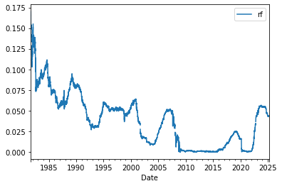
How do we interpret this rate?
Say if I invested in the tbill in 2005 how much money I would have in the end of 3 months? And in the end of the year?
Lets get another stock to play with and merge it together with our risk-free return
df=get_daily_wrds_single_ticker('NVDA',conn,dividends=False)
df=df.merge(df_rf, left_index=True, right_index=True,how='left')
df
[86580]
| ret | rf | |
|---|---|---|
| date | ||
| 1999-01-25 | 0.104762 | 0.0444 |
| 1999-01-26 | -0.077586 | 0.0446 |
| 1999-01-27 | -0.003115 | 0.0447 |
| 1999-01-28 | -0.003125 | 0.0449 |
| 1999-01-29 | -0.047022 | 0.0448 |
| ... | ... | ... |
| 2024-12-24 | 0.003938 | 0.0440 |
| 2024-12-26 | -0.002068 | 0.0435 |
| 2024-12-27 | -0.020868 | 0.0431 |
| 2024-12-30 | 0.003503 | 0.0437 |
| 2024-12-31 | -0.023275 | 0.0437 |
6527 rows × 2 columns
Lets construct another column called ‘ret_e’ for excess returns
What is the trading interpretation of such series?
Is it the “return” to which strategy exactly?
How the historical distributions of ret and rete compare?
Are their averages similar?
are their historical standard deviations similar?
Do they have similar interpretation?
Is the standard-deviation of risk-free rate useful to tell you the distribution of you returns in the end of 3 months for an investments in the risk-free asset?
4.3. Risk Premiums#
We call the risk-premium what we earn in excess of what a risk-free investment pays
So the risk premium of an asset is the expected value of the excess return
So the expected return of a stock is
The realized return is obviously volatile, hence the risk
will be negative 50% of the time and sometimes quite negative!
Big picture level the goal of quant investing is to harvest these risk-premia while managing the risk
We know the risk-free rate (it is the yield on a short-term government bond)
How do we figure out the risk-premium of an asset?
4.3.1. Stripping the common factor#
We will build a simple model to help us both think about this risk-premium and also the risk that we need to manage
It will be useful to decompose the excess returns further to better understand it’s risk and it’s premium
We know that the overall market portfolio moves around, so it is natural to strip that market-wide movement from the stock returns
Suppose f is this common factor, one possibility is to write
Reorganizing we have that the return can be written as
What is this common factor?
Will this work? When will it work?
I will use the returns on the SPY etf as a market proxy, i.e
This funds holds a market-capitalization weighted portfolio of the largest 500 US stocks (roughly)–this consists of about 85% of the total universe of investable US equities
The press often cites the DOW JONES as another proxy for the overall movement in stocks–but it is a terrible proxy, since is a equal weighted portfolio of 30 arbitrary chosen stocks. Please never ever use that
If you really want to use a portfolio that tracks the entirety of the US stock market universe you can use VTI which is a ETF that holds market-capitalization weighted portfolio of all publicly traded US stocks. About 60 Trillion investment universe
For reasons that will be clear later–but don’t matter for now, I will also strip the risk-free rate from our common factor
#conn = wrds.Connection()


df=get_daily_wrds(conn,tickers=['SPY','WMT','JPM'])
#Why did I divide by 252?
df=df.merge(df_rf/252, left_index=True, right_index=True,how='left')
df
[47896, 55976, 84398]
| SPY | WMT | JPM | rf | |
|---|---|---|---|---|
| date | ||||
| 1993-02-01 | 0.007112 | 0.011516 | 0.009231 | 0.000119 |
| 1993-02-02 | 0.002119 | 0.005693 | 0.003049 | 0.000120 |
| 1993-02-03 | 0.010571 | 0.009434 | 0.012158 | 0.000119 |
| 1993-02-04 | 0.004184 | -0.003738 | 0.012012 | 0.000117 |
| 1993-02-05 | -0.000694 | -0.011257 | 0.017804 | 0.000117 |
| ... | ... | ... | ... | ... |
| 2024-12-24 | 0.011115 | 0.025789 | 0.016444 | 0.000175 |
| 2024-12-26 | 0.000067 | 0.001187 | 0.003425 | 0.000173 |
| 2024-12-27 | -0.010527 | -0.012178 | -0.008102 | 0.000171 |
| 2024-12-30 | -0.011412 | -0.011892 | -0.007671 | 0.000173 |
| 2024-12-31 | -0.003638 | -0.002429 | 0.001630 | 0.000173 |
8037 rows × 4 columns
# will create excess retursn

df_re=df.drop(columns='rf').sub(df['rf'],axis=0)
df_re
| SPY | WMT | JPM | |
|---|---|---|---|
| date | |||
| 1993-02-01 | 0.006993 | 0.011397 | 0.009112 |
| 1993-02-02 | 0.001999 | 0.005573 | 0.002929 |
| 1993-02-03 | 0.010452 | 0.009315 | 0.012039 |
| 1993-02-04 | 0.004067 | -0.003855 | 0.011895 |
| 1993-02-05 | -0.000811 | -0.011374 | 0.017687 |
| ... | ... | ... | ... |
| 2024-12-24 | 0.010940 | 0.025614 | 0.016269 |
| 2024-12-26 | -0.000106 | 0.001014 | 0.003252 |
| 2024-12-27 | -0.010698 | -0.012349 | -0.008273 |
| 2024-12-30 | -0.011585 | -0.012065 | -0.007844 |
| 2024-12-31 | -0.003811 | -0.002602 | 0.001457 |
8037 rows × 3 columns
fig, axes = plt.subplots(1, 2, figsize=(18,6))
import statsmodels.api as sm


# Function to add regression line and beta coefficient

df_re.plot.scatter(x='SPY', y='WMT', ax=axes[0], title='SPY vs WMT')

# Scatter plot for SPY vs CSCO
df_re.plot.scatter(x='SPY', y='JPM', ax=axes[1], title='SPY vs JPM')

plt.tight_layout()
plt.show()
c:\Users\Alan.Moreira\Anaconda3\lib\site-packages\scipy\__init__.py:146: UserWarning: A NumPy version >=1.16.5 and <1.23.0 is required for this version of SciPy (detected version 1.26.0
  warnings.warn(f"A NumPy version >={np_minversion} and <{np_maxversion}"
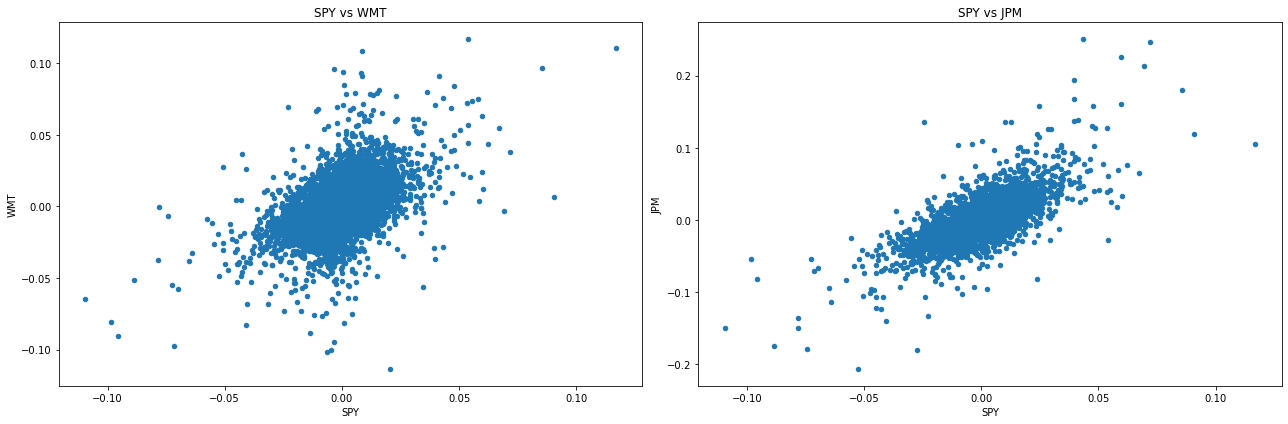
Indeed we see quite a bit of co-movement!
Days that SPY return is up, Both stocks tend to be up as well
Another way of see this is looking at the correlation between the stocks and the factor
df_re.corr()
| SPY | WMT | JPM | |
|---|---|---|---|
| SPY | 1.000000 | 0.492221 | 0.707302 |
| WMT | 0.492221 | 1.000000 | 0.325104 |
| JPM | 0.707302 | 0.325104 | 1.000000 |
Lets try to clean the stock from exposure to the common factor by subtracting it out
‘m_spy’ denote the returns minus the return on the factor
df_re[['WMT_m_spy','JPM_m_spy']]=df_re[['WMT','JPM']].subtract(df['SPY'],axis=0)
df
| SPY | WMT | JPM | rf | |
|---|---|---|---|---|
| date | ||||
| 1993-02-01 | 0.007112 | 0.011516 | 0.009231 | 0.000119 |
| 1993-02-02 | 0.002119 | 0.005693 | 0.003049 | 0.000120 |
| 1993-02-03 | 0.010571 | 0.009434 | 0.012158 | 0.000119 |
| 1993-02-04 | 0.004184 | -0.003738 | 0.012012 | 0.000117 |
| 1993-02-05 | -0.000694 | -0.011257 | 0.017804 | 0.000117 |
| ... | ... | ... | ... | ... |
| 2024-12-24 | 0.011115 | 0.025789 | 0.016444 | 0.000175 |
| 2024-12-26 | 0.000067 | 0.001187 | 0.003425 | 0.000173 |
| 2024-12-27 | -0.010527 | -0.012178 | -0.008102 | 0.000171 |
| 2024-12-30 | -0.011412 | -0.011892 | -0.007671 | 0.000173 |
| 2024-12-31 | -0.003638 | -0.002429 | 0.001630 | 0.000173 |
8037 rows × 4 columns
What is the trading interpretation in this case? What is the portfolio that yields the ‘ret_m_spy’ payoff?
What is the cost of implementing this portfolio? Say you want to have a 100 dollar exposure to it?
fig, axes = plt.subplots(1, 2, figsize=(18,6))
import statsmodels.api as sm


# Function to add regression line and beta coefficient

df_re.plot.scatter(x='SPY', y='WMT_m_spy', ax=axes[0], title='SPY vs WMT')

# Scatter plot for SPY vs CSCO
df_re.plot.scatter(x='SPY', y='JPM_m_spy', ax=axes[1], title='SPY vs JPM')

plt.tight_layout()
plt.show()
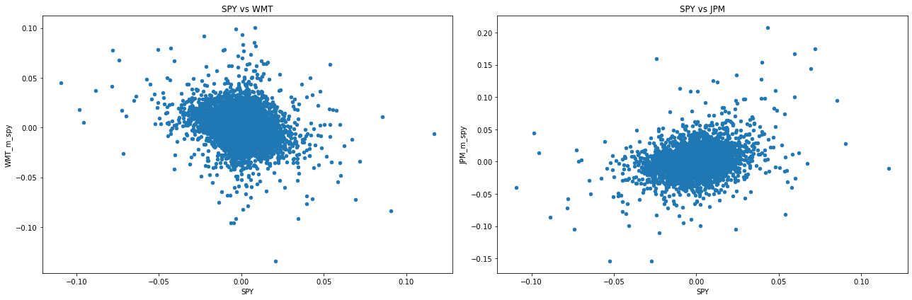
Did it work?
df_re.corr().loc['SPY',:]
SPY          1.000000
WMT          0.492221
JPM          0.707302
WMT_m_spy   -0.264076
JPM_m_spy    0.272552
Name: SPY, dtype: float64
df_re.std()
SPY          0.011617
WMT          0.015902
JPM          0.022911
WMT_m_spy    0.014351
JPM_m_spy    0.016833
dtype: float64
What is going on?
The “model” motivating our decomposition was
with the \(r-f-rf\) picking up the stock specific movement and \(f\) the common movement
But it seems that the residual still has factor exposure
For stock 1, the residual is negatively correlated, so it seems tha we are taking out too much
For stock 2, it is still positive, so we are taking out too little
Taking out 1 dollar of factor exposure for each 1 dollar of stock exposure reduced the factor exposure and the asset volatilities, but we can do better
What should we do? How do we fix this?
📝 Key Takeaways
Return = price change + income, normalized. Whether for stocks, bonds, or crypto, total return compares what you end with to what you put in.
Excess return is the correct performance yardstick. Subtracting the risk-free rate lets you focus on compensation for taking risk, not for simply waiting.
Risk premiums are expectations, not guarantees. The historical average of excess returns is noisy and must be interpreted with care.
Stocks do not share the same market sensitivity. Removing one dollar of market exposure from each asset under- or over-hedges depending on its true beta.