
3.4. Pandas#
3.4.1. Introduction#
import pandas as pd


%matplotlib inline
This lecture begins the material on pandas which is the library that allows us to work with data
To start, we will import the pandas package and give it the alias
pd, which is conventional practice.
There are two types of collections: Series, for a single variable, that is one columns with multiple rows, and a DataFrame, for multiple variables , that is multiple rows and columns
3.4.1.1. Series#
The first main pandas type we will introduce is called Series.
A Series is a single column of data, with row labels for each observation.
pandas refers to the row labels as the index of the Series.

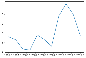
Below, we create a Series which contains the Google Stock price every other year starting in 2005. ( This is made up!)
# this creates a lsit with the stock prices of google from 2005 to 2015
values = [5.6, 5.3, 4.3, 4.2, 5.8, 5.3, 4.6, 7.8, 9.1, 8., 5.7]
# this creates a list with the years from 2005 to 2015
years = list(range(2005, 2016, 1))
# this creates a pandas series with the stock prices of google from 2005 to 2015

Google = pd.Series(data=values, index=years, name="Google Stock Price")

# lets see what it looks like
Google
We can look at the index and values in our Series.
Google.index
Int64Index([1995, 1997, 1999, 2001, 2003, 2005, 2007, 2009, 2011, 2013, 2015], dtype='int64')
Google.values
array([5.6, 5.3, 4.3, 4.2, 5.8, 5.3, 4.6, 7.8, 9.1, 8. , 5.7])
3.4.1.1.1. What Can We Do with a Series object?#
.head and .tail
Often, our data will have many rows, and we won’t want to display it all at once.
The methods .head and .tail show rows at the beginning and end
of our Series, respectively.
Google.head()
1995    5.6
1997    5.3
1999    4.3
2001    4.2
2003    5.8
Name: Unemployment, dtype: float64
Google.tail()
2007    4.6
2009    7.8
2011    9.1
2013    8.0
2015    5.7
Name: Unemployment, dtype: float64
3.4.1.2. Basic Plotting#
We can also plot data using the .plot method.
Google.plot()
<AxesSubplot:>
Note
This is why we needed the
%matplotlib inline— it tells the notebook to display figures inside the notebook itself. Also, pandas has much greater visualization functionality than this, but we will study that later on.
3.4.1.3. Indexing#
Sometimes, we will want to select particular elements from a Series.
We can do this using .loc[index_items]; where index_items is
an item from the index, or a list of items in the index.
We will see this more in-depth in a coming lecture, but for now, we demonstrate how to select one or multiple elements of the Series.
Google.loc[2007]
4.3
Google.loc[[2008, 2010, 2015]]
2008    4.2
2010    5.3
2015    5.7
Name: Google Stock Price, dtype: float64
3.4.1.4. DataFrame#
A DataFrame is how pandas stores one or more columns of data.
We can think a DataFrames a multiple Series stacked side by side as columns.
This is similar to a sheet in an Excel workbook or a table in a SQL database.
In addition to row labels (an index), DataFrames also have column labels.
We refer to these column labels as the columns or column names.

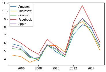
Below, we create a DataFrame that contains the Stock price in the end of each year starting in 2005 for a few US tech stocks.
(This is made up)
# create dictionary with stock prices of google, apple, amazon, microsoft, and facebook
#
data = {
    "Amazon": [5.9,  5.6,  4.4,  3.8,  5.8,  4.9,  4.3,  7.1,  8.3,  7.9,  5.7],
    "Microsoft": [4.5,  4.3,  3.6,  4. ,  5.7,  5.7,  4.9,  8.1,  8.7,  7.4,  5.1],
    "Google": [5.3,  5.2,  4.2,  4. ,  5.7,  5.2,  4.3,  7.6,  9.1,  7.4,  5.5],
    "Facebook": [6.6, 6., 5.2, 4.6, 6.5, 5.5, 4.5, 8.6, 10.7, 8.5, 6.1],
    "Apple": [5.6, 5.3, 4.3, 4.2, 5.8, 5.3, 4.6, 7.8, 9.1, 8., 5.7]
}

# create a pandas dataframe with the stock prices of google, apple, amazon, microsoft, and facebook
stock_prices = pd.DataFrame(data, index=years)
stock_prices
| Amazon | Microsoft | Apple | |||
|---|---|---|---|---|---|
| 2005 | 5.9 | 4.5 | 5.3 | 6.6 | 5.6 |
| 2006 | 5.6 | 4.3 | 5.2 | 6.0 | 5.3 |
| 2007 | 4.4 | 3.6 | 4.2 | 5.2 | 4.3 |
| 2008 | 3.8 | 4.0 | 4.0 | 4.6 | 4.2 |
| 2009 | 5.8 | 5.7 | 5.7 | 6.5 | 5.8 |
| 2010 | 4.9 | 5.7 | 5.2 | 5.5 | 5.3 |
| 2011 | 4.3 | 4.9 | 4.3 | 4.5 | 4.6 |
| 2012 | 7.1 | 8.1 | 7.6 | 8.6 | 7.8 |
| 2013 | 8.3 | 8.7 | 9.1 | 10.7 | 9.1 |
| 2014 | 7.9 | 7.4 | 7.4 | 8.5 | 8.0 |
| 2015 | 5.7 | 5.1 | 5.5 | 6.1 | 5.7 |
This is one way to create a dataframe
We can retrieve the index and the DataFrame values as we did with a Series.
stock_prices.index
Int64Index([2005, 2006, 2007, 2008, 2009, 2010, 2011, 2012, 2013, 2014, 2015], dtype='int64')
stock_prices.values
array([[ 5.9,  4.5,  5.3,  6.6,  5.6],
       [ 5.6,  4.3,  5.2,  6. ,  5.3],
       [ 4.4,  3.6,  4.2,  5.2,  4.3],
       [ 3.8,  4. ,  4. ,  4.6,  4.2],
       [ 5.8,  5.7,  5.7,  6.5,  5.8],
       [ 4.9,  5.7,  5.2,  5.5,  5.3],
       [ 4.3,  4.9,  4.3,  4.5,  4.6],
       [ 7.1,  8.1,  7.6,  8.6,  7.8],
       [ 8.3,  8.7,  9.1, 10.7,  9.1],
       [ 7.9,  7.4,  7.4,  8.5,  8. ],
       [ 5.7,  5.1,  5.5,  6.1,  5.7]])
What Can We Do with a DataFrame?
A lot stuff!
This will be the main way we will work with data in Python
3.4.1.4.1. .head and .tail#
As with Series, we can use .head and .tail to show only the
first or last n rows.
stock_prices.head()
| Amazon | Microsoft | Apple | |||
|---|---|---|---|---|---|
| 2005 | 5.9 | 4.5 | 5.3 | 6.6 | 5.6 |
| 2006 | 5.6 | 4.3 | 5.2 | 6.0 | 5.3 |
| 2007 | 4.4 | 3.6 | 4.2 | 5.2 | 4.3 |
| 2008 | 3.8 | 4.0 | 4.0 | 4.6 | 4.2 |
| 2009 | 5.8 | 5.7 | 5.7 | 6.5 | 5.8 |
3.4.1.5. Plotting#
We can generate plots with the .plot method.
Notice we now have a separate line for each column of data.
stock_prices.plot()
<AxesSubplot:>
3.4.2. Indexing#
We can also do indexing using .loc.
This is slightly more advanced than before because we can choose subsets of both row and columns.
stock_prices.loc[2005, "Apple"]
5.6
stock_prices.loc[[2005,2008], "Facebook"]
2005    6.6
2008    4.6
Name: Facebook, dtype: float64
stock_prices.loc[2005, ["Microsoft", "Google"]]
Microsoft    4.5
Google       5.3
Name: 2005, dtype: float64
stock_prices.loc[:, "Microsoft"]
2005    4.5
2006    4.3
2007    3.6
2008    4.0
2009    5.7
2010    5.7
2011    4.9
2012    8.1
2013    8.7
2014    7.4
2015    5.1
Name: Microsoft, dtype: float64
# `[string]` with no `.loc` extracts a whole column
stock_prices["Apple"]
2005    5.6
2006    5.3
2007    4.3
2008    4.2
2009    5.8
2010    5.3
2011    4.6
2012    7.8
2013    9.1
2014    8.0
2015    5.7
Name: Apple, dtype: float64
3.4.2.1. Computations with Columns#
pandas can do various computations and mathematical operations on columns.
Let’s take a look at a few of them.
# Divide by 100
stock_prices / 100
| Amazon | Microsoft | Apple | |||
|---|---|---|---|---|---|
| 2005 | 0.059 | 0.045 | 0.053 | 0.066 | 0.056 |
| 2006 | 0.056 | 0.043 | 0.052 | 0.060 | 0.053 |
| 2007 | 0.044 | 0.036 | 0.042 | 0.052 | 0.043 |
| 2008 | 0.038 | 0.040 | 0.040 | 0.046 | 0.042 |
| 2009 | 0.058 | 0.057 | 0.057 | 0.065 | 0.058 |
| 2010 | 0.049 | 0.057 | 0.052 | 0.055 | 0.053 |
| 2011 | 0.043 | 0.049 | 0.043 | 0.045 | 0.046 |
| 2012 | 0.071 | 0.081 | 0.076 | 0.086 | 0.078 |
| 2013 | 0.083 | 0.087 | 0.091 | 0.107 | 0.091 |
| 2014 | 0.079 | 0.074 | 0.074 | 0.085 | 0.080 |
| 2015 | 0.057 | 0.051 | 0.055 | 0.061 | 0.057 |
# Find maximum
stock_prices["Apple"].max()
9.1
# Find the difference between two columns
# Notice that pandas applies `-` to _all rows_ at once
# We'll see more of this throughout these materials
stock_prices["Google"] - stock_prices["Apple"]
2005   -0.3
2006   -0.1
2007   -0.1
2008   -0.2
2009   -0.1
2010   -0.1
2011   -0.3
2012   -0.2
2013    0.0
2014   -0.6
2015   -0.2
dtype: float64
# Find correlation between two columns
stock_prices['Apple'].corr(stock_prices["Microsoft"])
0.9523890760029825
# find correlation between all column pairs
stock_prices.corr()
| Amazon | Microsoft | Apple | |||
|---|---|---|---|---|---|
| Amazon | 1.000000 | 0.875654 | 0.964415 | 0.967875 | 0.976016 |
| Microsoft | 0.875654 | 1.000000 | 0.951379 | 0.900638 | 0.952389 |
| 0.964415 | 0.951379 | 1.000000 | 0.987259 | 0.995030 | |
| 0.967875 | 0.900638 | 0.987259 | 1.000000 | 0.981308 | |
| Apple | 0.976016 | 0.952389 | 0.995030 | 0.981308 | 1.000000 |
3.4.2.2. Data Types#
We asked you to run the commands unemp.dtype and
unemp_region.dtypes and think about the outputs.
You might have guessed that they return the type of the values inside each column.
Occasionally, you might need to investigate what types you have in your DataFrame when an operation isn’t behaving as expected.
Google.dtype
dtype('float64')
stock_prices.dtypes
Amazon       float64
Microsoft    float64
Google       float64
Facebook     float64
Apple        float64
dtype: object
DataFrames will only distinguish between a few types.
Booleans (
bool)Floating point numbers (
float64)Integers (
int64)Dates (
datetime) — we will learn this soonCategorical data (
categorical)Everything else, including strings (
object)
In the future, we will often refer to the type of data stored in a
column as its dtype.
Let’s look at an example for when having an incorrect dtype can
cause problems.
Suppose that when we imported the data the South column was
interpreted as a string.
stock_prices_str = stock_prices.copy()
stock_prices_str["Apple"] = stock_prices_str["Apple"].astype(str)
stock_prices_str.dtypes
Amazon       float64
Microsoft    float64
Google       float64
Facebook     float64
Apple         object
dtype: object
Everything looks ok…
stock_prices_str.head()
| Amazon | Microsoft | Apple | |||
|---|---|---|---|---|---|
| 2005 | 5.9 | 4.5 | 5.3 | 6.6 | 5.6 |
| 2006 | 5.6 | 4.3 | 5.2 | 6.0 | 5.3 |
| 2007 | 4.4 | 3.6 | 4.2 | 5.2 | 4.3 |
| 2008 | 3.8 | 4.0 | 4.0 | 4.6 | 4.2 |
| 2009 | 5.8 | 5.7 | 5.7 | 6.5 | 5.8 |
But if we try to do something like compute the sum of all the columns, we get unexpected results…
stock_prices_str.sum()
Amazon                                    63.7
Microsoft                                 62.0
Google                                    63.5
Facebook                                  72.8
Apple        5.65.34.34.25.85.34.67.89.18.05.7
dtype: object
Why this happened?
3.4.2.3. Changing DataFrames#
We can change the data inside of a DataFrame in various ways:
Adding new columns
Changing index labels or column names
Altering existing data (e.g. doing some arithmetic or making a column of strings lowercase)
3.4.2.4. Creating New Columns#
We can create new data by assigning values to a column similar to how we assign values to a variable.
In pandas, we create a new column of a DataFrame by writing:
df["New Column Name"] = new_values
Below, we create an unweighted mean of the unemployment rate across the four regions of the US — notice that this differs from the national unemployment rate.
stock_prices["ValueofEW_portfolio"] = (stock_prices["Amazon"] +
                                  stock_prices["Apple"] +
                                  stock_prices["Microsoft"] +
                                  stock_prices["Google"]+
                                  stock_prices['Facebook'])/5

# what is a easier way to accomplish this?
stock_prices.head()
| Amazon | Microsoft | Apple | ValueofEW_portfolio | |||
|---|---|---|---|---|---|---|
| 2005 | 5.9 | 4.5 | 5.3 | 6.6 | 5.6 | 5.58 |
| 2006 | 5.6 | 4.3 | 5.2 | 6.0 | 5.3 | 5.28 |
| 2007 | 4.4 | 3.6 | 4.2 | 5.2 | 4.3 | 4.34 |
| 2008 | 3.8 | 4.0 | 4.0 | 4.6 | 4.2 | 4.12 |
| 2009 | 5.8 | 5.7 | 5.7 | 6.5 | 5.8 | 5.90 |
3.4.2.5. Changing Values#
Changing the values inside of a DataFrame should be done very rarely.
Typically when you are using the dataframe to store some computation
However, it can be done by assigning a value to a location in the DataFrame.
df.loc[index, column] = value
stock_prices.loc[2015, "ValueofEW_portfolio"] = 0.0
stock_prices.tail()
| Amazon | Microsoft | Apple | ValueofEW_portfolio | |||
|---|---|---|---|---|---|---|
| 2011 | 4.3 | 4.9 | 4.3 | 4.5 | 4.6 | 4.52 |
| 2012 | 7.1 | 8.1 | 7.6 | 8.6 | 7.8 | 7.84 |
| 2013 | 8.3 | 8.7 | 9.1 | 10.7 | 9.1 | 9.18 |
| 2014 | 7.9 | 7.4 | 7.4 | 8.5 | 8.0 | 7.84 |
| 2015 | 5.7 | 5.1 | 5.5 | 6.1 | 5.7 | 0.00 |
3.4.2.6. Renaming Columns#
We can also rename the columns of a DataFrame, which is helpful because the names that sometimes come with datasets are unbearable…
For example, twe can change facebook to Meta and google became alphabet.
We can rename columns by passing a dictionary to the rename method.
This dictionary contains the old names as the keys and new names as the values.
See the example below.
names = {"Facebook": "Meta",
         "Google": "Alphabet"}
stock_prices.rename(columns=names)
| Amazon | Microsoft | Alphabet | Meta | Apple | ValueofEW_portfolio | |
|---|---|---|---|---|---|---|
| 2005 | 5.9 | 4.5 | 5.3 | 6.6 | 5.6 | 5.58 |
| 2006 | 5.6 | 4.3 | 5.2 | 6.0 | 5.3 | 5.28 |
| 2007 | 4.4 | 3.6 | 4.2 | 5.2 | 4.3 | 4.34 |
| 2008 | 3.8 | 4.0 | 4.0 | 4.6 | 4.2 | 4.12 |
| 2009 | 5.8 | 5.7 | 5.7 | 6.5 | 5.8 | 5.90 |
| 2010 | 4.9 | 5.7 | 5.2 | 5.5 | 5.3 | 5.32 |
| 2011 | 4.3 | 4.9 | 4.3 | 4.5 | 4.6 | 4.52 |
| 2012 | 7.1 | 8.1 | 7.6 | 8.6 | 7.8 | 7.84 |
| 2013 | 8.3 | 8.7 | 9.1 | 10.7 | 9.1 | 9.18 |
| 2014 | 7.9 | 7.4 | 7.4 | 8.5 | 8.0 | 7.84 |
| 2015 | 5.7 | 5.1 | 5.5 | 6.1 | 5.7 | 0.00 |
stock_prices.head()
| Amazon | Microsoft | Apple | ValueofEW_portfolio | |||
|---|---|---|---|---|---|---|
| 2005 | 5.9 | 4.5 | 5.3 | 6.6 | 5.6 | 5.58 |
| 2006 | 5.6 | 4.3 | 5.2 | 6.0 | 5.3 | 5.28 |
| 2007 | 4.4 | 3.6 | 4.2 | 5.2 | 4.3 | 4.34 |
| 2008 | 3.8 | 4.0 | 4.0 | 4.6 | 4.2 | 4.12 |
| 2009 | 5.8 | 5.7 | 5.7 | 6.5 | 5.8 | 5.90 |
We renamed our columns… Why does the DataFrame still show the old column names?
Many pandas operations create a copy of your data by default to protect your data and prevent you from overwriting information you meant to keep.
We can make these operations permanent by either:
Assigning the output back to the variable name
df = df.rename(columns=rename_dict)Looking into whether the method has an
inplaceoption. For example,df.rename(columns=rename_dict, inplace=True)
Setting inplace=True will sometimes make your code faster
(e.g. if you have a very large DataFrame and you don’t want to copy all
the data), but that doesn’t always happen.
We recommend using the first option until you get comfortable with pandas because operations that don’t alter your data are (usually) safer.
names = {"Facebook": "Meta",
         "Google": "Alphabet"}
stock_prices=stock_prices.rename(columns=names)
stock_prices.head()
| Amazon | Microsoft | Alphabet | Meta | Apple | ValueofEW_portfolio | |
|---|---|---|---|---|---|---|
| 2005 | 5.9 | 4.5 | 5.3 | 6.6 | 5.6 | 5.58 |
| 2006 | 5.6 | 4.3 | 5.2 | 6.0 | 5.3 | 5.28 |
| 2007 | 4.4 | 3.6 | 4.2 | 5.2 | 4.3 | 4.34 |
| 2008 | 3.8 | 4.0 | 4.0 | 4.6 | 4.2 | 4.12 |
| 2009 | 5.8 | 5.7 | 5.7 | 6.5 | 5.8 | 5.90 |
3.4.2.7. Dates in pandas#
Now lets understand date manipulation more carefully
So far our years were integer, but to work with dates it is convenient to have data type specific for it
In pandas this type is datetime
LEts import a monthly data set with returns of 50 different companies
url = "https://raw.githubusercontent.com/amoreira2/Fin418/main/assets/data/Retuns50stocks.csv"
df_returns50 = pd.read_csv(url)
df_returns50
| date | CTL | T | CSCO | FCX | XL | IVZ | AMT | WHR | IR | ... | SWK | DVN | TMO | PEP | LNC | EMR | MLM | CCI | NU | Market | |
|---|---|---|---|---|---|---|---|---|---|---|---|---|---|---|---|---|---|---|---|---|---|
| 0 | 200001 | -18.4697 | -11.5513 | 2.2170 | -17.4556 | -12.5301 | -4.0929 | 17.3824 | -10.4707 | -14.5289 | ... | -16.5975 | 6.8441 | 15.4167 | -3.1915 | -6.9312 | -4.0305 | 2.4390 | -1.5564 | -0.3040 | -3.9612 |
| 1 | 200002 | -12.9450 | -11.2245 | 20.7192 | -21.1470 | -9.8898 | 5.3057 | 37.2822 | -6.1760 | -18.2311 | ... | -8.4577 | 6.0498 | -9.7473 | -5.8608 | -25.2115 | -16.6039 | -15.1667 | 1.9763 | -7.7439 | 3.1777 |
| 2 | 200003 | 10.5502 | 10.6732 | 16.9740 | -12.2727 | 36.9397 | 24.4250 | 0.2538 | 7.9402 | 15.4976 | ... | 15.6304 | 30.5034 | 30.4000 | 8.9805 | 21.2670 | 16.5981 | 33.8028 | 17.4419 | 14.2857 | 5.3500 |
| 3 | 200004 | -34.0067 | 4.6083 | -10.3274 | -20.2073 | -13.9955 | 0.9670 | -5.6962 | 11.0874 | 6.0734 | ... | 11.8483 | -0.9009 | -4.9080 | 5.1971 | 4.7836 | 3.2941 | 11.5789 | 1.3201 | 0.0000 | -5.9530 |
| 4 | 200005 | 10.3980 | -0.2853 | -17.8724 | -4.5455 | 25.8793 | -8.7719 | -20.2685 | -12.4338 | -2.5672 | ... | -8.8983 | 24.2857 | -4.1935 | 11.4140 | 11.3106 | 8.1686 | -7.4198 | -31.7590 | 3.3721 | -3.8871 |
| ... | ... | ... | ... | ... | ... | ... | ... | ... | ... | ... | ... | ... | ... | ... | ... | ... | ... | ... | ... | ... | ... |
| 175 | 201408 | 5.8359 | -1.7702 | -0.9512 | -2.2837 | 6.0174 | 9.1948 | 4.4602 | 7.8029 | 2.3984 | ... | 4.6312 | -0.1060 | -1.0617 | 4.9830 | 5.0582 | 1.2569 | 5.7394 | 7.1852 | 4.5330 | 4.0171 |
| 176 | 201409 | -0.2440 | 0.8009 | 1.4806 | -10.2282 | -2.4868 | -3.3301 | -4.6755 | -4.8164 | -5.9635 | ... | -2.3934 | -9.2814 | 1.3643 | 1.3569 | -2.6526 | -2.2493 | -1.5425 | 1.7230 | -2.6095 | -2.5129 |
| 177 | 201410 | 1.4429 | 0.1703 | -2.7811 | -11.7534 | 2.1405 | 2.5076 | 4.1333 | 18.1257 | 11.1072 | ... | 5.4623 | -11.9977 | -3.3936 | 3.3086 | 2.5009 | 2.3650 | -9.3222 | -2.9927 | 11.3995 | 2.1178 |
| 178 | 201411 | -0.4098 | 1.5499 | 12.9546 | -5.7895 | 4.8406 | 0.3459 | 7.7026 | 8.6428 | 0.7027 | ... | 0.8543 | -1.7167 | 9.9685 | 4.0865 | 3.4149 | 0.2498 | 3.0106 | 6.3620 | 2.6140 | 2.1149 |
| 179 | 201412 | -2.9188 | -5.0594 | 0.6331 | -12.9981 | -2.7872 | -2.0813 | -5.5042 | 4.0662 | 0.9198 | ... | 2.2872 | 4.2055 | -2.9778 | -4.8801 | 1.8365 | -3.1686 | -8.0973 | -4.2965 | 6.4623 | -0.3616 |
180 rows × 52 columns
Note that the data was not imported correctly
df_returns50.info()
<class 'pandas.core.frame.DataFrame'>
RangeIndex: 180 entries, 0 to 179
Data columns (total 52 columns):
 #   Column  Non-Null Count  Dtype
---  ------  --------------  -----
 0   date    180 non-null    int64
 1   CTL     180 non-null    float64
 2   T       180 non-null    float64
 3   CSCO    180 non-null    float64
 4   FCX     180 non-null    float64
 5   XL      180 non-null    float64
 6   IVZ     180 non-null    float64
 7   AMT     180 non-null    float64
 8   WHR     180 non-null    float64
 9   IR      180 non-null    float64
 10  WFT     180 non-null    float64
 11  YUM     180 non-null    float64
 12  CVS     180 non-null    float64
 13  GD      180 non-null    float64
 14  TYC     180 non-null    float64
 15  EL      180 non-null    float64
 16  MUR     180 non-null    float64
 17  CTAS    180 non-null    float64
 18  CBSA    180 non-null    float64
 19  SNV     180 non-null    float64
 20  CAM     180 non-null    float64
 21  DLTR    180 non-null    float64
 22  CAH     180 non-null    float64
 23  DTE     180 non-null    float64
 24  SSP     180 non-null    float64
 25  PSA     180 non-null    float64
 26  EXC     180 non-null    float64
 27  TKR     180 non-null    float64
 28  CMA     180 non-null    float64
 29  ORCL    180 non-null    float64
 30  MS      180 non-null    float64
 31  RSG     180 non-null    float64
 32  ACAS    180 non-null    float64
 33  AGN     180 non-null    float64
 34  MMM     180 non-null    float64
 35  ETFC    180 non-null    float64
 36  CAR     180 non-null    float64
 37  MDR     180 non-null    float64
 38  NOV     180 non-null    float64
 39  PCH     180 non-null    float64
 40  BAX     180 non-null    float64
 41  JCI     180 non-null    float64
 42  SWK     180 non-null    float64
 43  DVN     180 non-null    float64
 44  TMO     180 non-null    float64
 45  PEP     180 non-null    float64
 46  LNC     180 non-null    float64
 47  EMR     180 non-null    float64
 48  MLM     180 non-null    float64
 49  CCI     180 non-null    float64
 50  NU      180 non-null    float64
 51  Market  180 non-null    float64
dtypes: float64(51), int64(1)
memory usage: 73.2 KB
from datetime import datetime

# Create a date parser function that will allow pandas to read the dates in the format we have them
date_parser = lambda x: datetime.strptime(x, "%Y%m")

# Use pd.read_csv with the date_parser
df_returns50  = pd.read_csv(url, parse_dates=['date'], date_parser=date_parser)
df_returns50.info()
<class 'pandas.core.frame.DataFrame'>
RangeIndex: 180 entries, 0 to 179
Data columns (total 52 columns):
 #   Column  Non-Null Count  Dtype
---  ------  --------------  -----
 0   date    180 non-null    datetime64[ns]
 1   CTL     180 non-null    float64
 2   T       180 non-null    float64
 3   CSCO    180 non-null    float64
 4   FCX     180 non-null    float64
 5   XL      180 non-null    float64
 6   IVZ     180 non-null    float64
 7   AMT     180 non-null    float64
 8   WHR     180 non-null    float64
 9   IR      180 non-null    float64
 10  WFT     180 non-null    float64
 11  YUM     180 non-null    float64
 12  CVS     180 non-null    float64
 13  GD      180 non-null    float64
 14  TYC     180 non-null    float64
 15  EL      180 non-null    float64
 16  MUR     180 non-null    float64
 17  CTAS    180 non-null    float64
 18  CBSA    180 non-null    float64
 19  SNV     180 non-null    float64
 20  CAM     180 non-null    float64
 21  DLTR    180 non-null    float64
 22  CAH     180 non-null    float64
 23  DTE     180 non-null    float64
 24  SSP     180 non-null    float64
 25  PSA     180 non-null    float64
 26  EXC     180 non-null    float64
 27  TKR     180 non-null    float64
 28  CMA     180 non-null    float64
 29  ORCL    180 non-null    float64
 30  MS      180 non-null    float64
 31  RSG     180 non-null    float64
 32  ACAS    180 non-null    float64
 33  AGN     180 non-null    float64
 34  MMM     180 non-null    float64
 35  ETFC    180 non-null    float64
 36  CAR     180 non-null    float64
 37  MDR     180 non-null    float64
 38  NOV     180 non-null    float64
 39  PCH     180 non-null    float64
 40  BAX     180 non-null    float64
 41  JCI     180 non-null    float64
 42  SWK     180 non-null    float64
 43  DVN     180 non-null    float64
 44  TMO     180 non-null    float64
 45  PEP     180 non-null    float64
 46  LNC     180 non-null    float64
 47  EMR     180 non-null    float64
 48  MLM     180 non-null    float64
 49  CCI     180 non-null    float64
 50  NU      180 non-null    float64
 51  Market  180 non-null    float64
dtypes: datetime64[ns](1), float64(51)
memory usage: 73.2 KB
# Set the date column as the index
df_returns50.set_index("date", inplace=True)
df_returns50.index
DatetimeIndex(['2000-01-01', '2000-02-01', '2000-03-01', '2000-04-01',
               '2000-05-01', '2000-06-01', '2000-07-01', '2000-08-01',
               '2000-09-01', '2000-10-01',
               ...
               '2014-03-01', '2014-04-01', '2014-05-01', '2014-06-01',
               '2014-07-01', '2014-08-01', '2014-09-01', '2014-10-01',
               '2014-11-01', '2014-12-01'],
              dtype='datetime64[ns]', name='date', length=180, freq=None)
We can index into a DataFrame with a DatetimeIndex using string
representations of dates.
For example
# Data corresponding to a single date
df_returns50.loc["2005-01", :]
| CTL | T | CSCO | FCX | XL | IVZ | AMT | WHR | IR | WFT | ... | SWK | DVN | TMO | PEP | LNC | EMR | MLM | CCI | NU | Market | |
|---|---|---|---|---|---|---|---|---|---|---|---|---|---|---|---|---|---|---|---|---|---|
| date | |||||||||||||||||||||
| 2005-01-01 | -8.0914 | -6.5483 | -6.6253 | -3.0604 | -3.6961 | 7.0064 | -1.5217 | -1.3726 | -7.3724 | 5.7895 | ... | -2.919 | 4.4964 | -0.8281 | 2.8736 | -0.3749 | -4.0799 | 0.6709 | -1.4423 | -0.7958 | -2.6552 |
1 rows × 51 columns
# Data for all days between New Years Day and June first in the year 2000
df_returns50.loc["01/2003":"06/2003", :]
| CTL | T | CSCO | FCX | XL | IVZ | AMT | WHR | IR | WFT | ... | SWK | DVN | TMO | PEP | LNC | EMR | MLM | CCI | NU | Market | |
|---|---|---|---|---|---|---|---|---|---|---|---|---|---|---|---|---|---|---|---|---|---|
| date | |||||||||||||||||||||
| 2003-01-01 | 3.233500 | -8.8528 | 2.0611 | 11.8594 | -2.8350 | -8.3333 | 43.9093 | -0.4787 | -8.8249 | -6.9371 | ... | -23.0191 | -1.3072 | -9.6919 | -4.1213 | 3.182400 | -7.708899 | -4.7619 | 5.3333 | -5.4054 | -2.3392 |
| 2003-02-01 | -9.660399 | -14.8936 | 4.5625 | -9.3234 | -5.4889 | -18.9610 | -7.6772 | -4.5603 | 0.9170 | 7.7503 | ... | -3.0428 | 6.4018 | -3.1370 | -5.3360 | -12.155000 | 1.134700 | -5.0342 | -1.7722 | -1.4808 | -1.5390 |
| 2003-03-01 | 0.930700 | -3.5577 | -7.1531 | 0.1763 | 0.4511 | -2.3504 | 17.6972 | -0.4669 | -2.1800 | -5.6693 | ... | -6.0635 | 0.1452 | 2.8409 | 4.7756 | -1.164800 | -3.654100 | 0.1088 | 41.7526 | -0.5714 | 1.0325 |
| 2003-04-01 | 6.702900 | 18.1082 | 15.5624 | 2.0528 | 16.2758 | 24.0886 | 20.2899 | 9.0965 | 14.2265 | 6.5131 | ... | 0.1667 | -1.9079 | 0.3867 | 8.2000 | 15.339300 | 11.797100 | 7.0989 | 15.8182 | 7.1839 | 8.2762 |
| 2003-05-01 | 14.329400 | 8.9897 | 9.4000 | 26.8053 | 5.7716 | 11.4311 | 34.9398 | 7.0107 | -0.2496 | 12.7268 | ... | 17.4157 | 10.0529 | 16.1255 | 2.1257 | 8.886101 | 3.930000 | 16.3003 | 30.7692 | 9.2326 | 6.3471 |
| 2003-06-01 | 3.668000 | 0.3535 | 2.3157 | 11.6173 | -4.1011 | 12.9241 | -1.2277 | 11.9508 | 8.0365 | -7.6075 | ... | -1.2875 | 2.6923 | -0.3791 | 1.0407 | 2.385100 | -2.294500 | -1.7539 | -6.7227 | 3.5891 | 1.6336 |
6 rows × 51 columns
3.4.2.8. DataFrame Aggregations#
Let’s talk about aggregations.
Loosely speaking, an aggregation is an operation that combines multiple values into a single value.
For example, computing the mean of three numbers (for example
[0, 1, 2]) returns a single number (1).
We will use aggregations extensively as we analyze and manipulate our data.
Thankfully, pandas makes this easy!
3.4.2.8.1. Built-in Aggregations#
pandas already has some of the most frequently used aggregations.
For example:
Mean (
mean)Variance (
var)Standard deviation (
std)Minimum (
min)Median (
median)Maximum (
max)etc…
Note
When looking for common operations, using “tab completion” goes a long way.
df_returns50.mean()
CTL       0.543043
T         0.420712
CSCO      0.272205
FCX       1.562149
XL        0.795499
IVZ       1.184839
AMT       1.819912
WHR       1.448373
IR        1.238221
WFT       1.072977
YUM       1.521299
CVS       1.248207
GD        1.351494
TYC       0.860400
EL        1.022905
MUR       1.307606
CTAS      0.873001
CBSA      0.839838
SNV       0.333623
CAM       1.294745
DLTR      1.551786
CAH       1.056583
DTE       1.100076
SSP       1.682069
PSA       1.685901
EXC       0.931623
TKR       1.400294
CMA       0.592855
ORCL      0.836469
MS        0.489803
RSG       1.215401
ACAS      1.536324
AGN       1.527276
MMM       1.046845
ETFC      0.078211
CAR       2.628951
MDR       1.817811
NOV       2.050656
PCH       0.890657
BAX       0.921694
JCI       1.496786
SWK       1.201223
DVN       1.245351
TMO       1.574135
PEP       0.842792
LNC       1.240616
EMR       0.889204
MLM       1.019899
CCI       1.533439
NU        0.931297
Market    0.487743
dtype: float64
As seen above, the aggregation’s default is to aggregate each column.
However, by using the axis keyword argument, you can do aggregations by
row as well.
df_returns50.mean(axis=1)
date
2000-01-01    -3.620535
2000-02-01    -3.927663
2000-03-01    13.901192
2000-04-01     0.988890
2000-05-01     1.003367
                ...
2014-08-01     3.464653
2014-09-01    -3.517967
2014-10-01     1.356545
2014-11-01     1.745494
2014-12-01     0.175312
Length: 180, dtype: float64
What is the finance interpretation of the time-series above?
3.4.2.9. Transforms#
Many analytical operations do not necessarily involve an aggregation.
The output of a function applied to a Series might need to be a new Series.
Some examples:
Compute the percentage change in average firm size from month to month.
Calculate the cumulative sum of elements in each column.
3.4.2.9.1. Built-in Transforms#
pandas comes with many transform functions including:
Cumulative sum/max/min/product (
cum(sum|min|max|prod))Difference (
diff)Elementwise addition/subtraction/multiplication/division (
+,-,*,/)Percent change (
pct_change)Number of occurrences of each distinct value (
value_counts)Absolute value (
abs)
Again, tab completion is helpful when trying to find these functions.
How do I compute the cumulative return of an equal weighted portfolio of these stocks?
3.4.2.10. Boolean Selection#
We have seen how we can select subsets of data by referring to the index or column names.
However, we often want to select based on conditions met by the data itself.
Some examples are:
Restrict analysis to all individuals older than 18.
Look at data that corresponds to particular time periods.
Analyze only data that corresponds to a recession.
Obtain data for a specific product or customer ID.
We will be able to do this by using a Series or list of boolean values to index into a Series or DataFrame.
#lets find all dates that the CVS stock has a monthly return lower than -10%

df_returns50.loc[df_returns50["CVS"]<-10,"CVS"]
date
2000-01-01   -12.2382
2001-06-01   -29.6904
2001-10-01   -27.8389
2002-09-01   -13.7462
2005-10-01   -15.7316
2009-11-01   -12.1530
2010-06-01   -15.3335
2010-08-01   -12.0886
Name: CVS, dtype: float64
Suppose I want to see how another stock, say CSCO, performed in these dates.
What do I do?
What is happening behind the scenes is boolean selection
df_returns50["CVS"]<-10
date
2000-01-01     True
2000-02-01    False
2000-03-01    False
2000-04-01    False
2000-05-01    False
              ...
2014-08-01    False
2014-09-01    False
2014-10-01    False
2014-11-01    False
2014-12-01    False
Name: CVS, Length: 180, dtype: bool