Show code cell content

Hide code cell content

# load libraries
import numpy as np
import pandas as pd
%matplotlib inline
import matplotlib.pyplot as plt
import pandas_datareader.data as web
# define functions  
def get_daily_wrds(conn,tickers=None):
  
    # Retrieve PERMNOs for the specified tickers
    permnos = conn.get_table(library='crsp', table='stocknames', columns=['permno', 'ticker', 'namedt', 'nameenddt'])
    permnos['nameenddt']=pd.to_datetime(permnos['nameenddt'])
    permnos = permnos[(permnos['ticker'].isin(tickers)) & (permnos['nameenddt']==permnos['nameenddt'].max())]
    # Extract unique PERMNOs
    permno_list = permnos['permno'].unique().tolist()
    print(permno_list)

    # Query daily stock file for the specified PERMNOs
    
    query = f"""
        SELECT permno, date, ret, retx, prc       
        FROM crsp.dsf
        WHERE permno IN ({','.join(map(str, permno_list))})
        ORDER BY date,permno
    """
    daily_returns = conn.raw_sql(query, date_cols=['date'])
    daily_returns = daily_returns.merge(permnos[['permno', 'ticker']], on='permno', how='left')
# Pivot data to have dates as index and tickers as columns
    daily_returns = daily_returns.pivot(index='date', columns='ticker', values='ret')    
    daily_returns=daily_returns[tickers]

    return daily_returns


def get_factors(factors='CAPM'):   
    if factors=='CAPM':
        fama_french = web.DataReader("F-F_Research_Data_Factors_daily", "famafrench",start="1921-01-01")
        daily_data = fama_french[0]
        daily_data.index = pd.to_datetime(daily_data.index)
        df_factor = daily_data[['RF','Mkt-RF']] 
    elif factors=='FF3':
        fama_french = web.DataReader("F-F_Research_Data_Factors_daily", "famafrench",start="1921-01-01")
        daily_data = fama_french[0]
        daily_data.index = pd.to_datetime(daily_data.index)
        df_factor = daily_data[['RF','Mkt-RF','SMB','HML']]
    elif factors=='FF5':
        fama_french = web.DataReader("F-F_Research_Data_5_Factors_2x3_daily", "famafrench",start="1921-01-01")
        daily_data = fama_french[0]
        daily_data.index = pd.to_datetime(daily_data.index)
        df_factor = daily_data[['RF','Mkt-RF','SMB','HML','RMW','CMA']]
    else:
        fama_french = web.DataReader("F-F_Research_Data_5_Factors_2x3_daily", "famafrench",start="1921-01-01")
        daily_data = fama_french[0]
        daily_data.index = pd.to_datetime(daily_data.index)
        df_factor = daily_data[['RF','Mkt-RF','SMB','HML','RMW','CMA']]
        fama_french = web.DataReader("F-F_Momentum_Factor_daily", "famafrench",start="1921-01-01")
        df_factor=df_factor.merge(fama_french[0],on='Date')    

    return df_factor/100

8. Estimation: From historical data to the future dynamics of returns

---

🎯 Learning Objectives

By the end of this chapter, you should be able to:

1. The six inputs to a factor model
   List exactly what must be estimated to forecast an asset’s distribution—risk-free rate, beta, factor risk-premium, alpha, factor variance, idiosyncratic variance.

2. Estimate β accurately.
   Practice running rolling regressions and understand when a cross-section or a time-series approach delivers a more reliable exposure.

3. Measure variances two ways.
   Compare cross-sectional dispersion in a single month with time-series volatility of one asset; recognize when each view is informative.

4. Form expectations for factor risk-premia.
   Use long‐sample averages when premia are thought to be stable, and learn warning signs that the mean may have shifted.

5. Appreciate why “alpha is all you need”—and why it’s elusive.
   Recognize that true alpha is scarce, tends to decay quickly, and often disappears once too much capital piles in.

6. Identify practical paths to alpha.
   Examine valuation edge, liquidity-provision trades, and alternative data as real-world ways investors create forecastable idiosyncratic returns.

7. Standardize alpha across horizons.
   Convert any price target or event view into a monthly (or other chosen) alpha so different ideas can be compared on the same scale.

8. Guard against hidden macro bets.
   Test that a proposed alpha is not simply a disguised market or sector exposure; if it is, rethink whether hedging or a broader position is more efficient.

---

We have been working with a single asset, since factor model

Realized returns:

\[r=rf+\alpha + b(f-rf)+\epsilon\]

Expected returns

\[E[r]=rf+\alpha + b*E[f]\]

Expected excess returns

\[E[r^{e}]=\alpha + b*E[f]\]

Variance:

\[Var(r)=b^2Var(f-rf)+Var(\epsilon)\]

To know the expected returns of your investment you need

1. The risk-free rate

2. The beta

3. The factor risk-premia

4. The asset specific alpha

To know the risk/variance of your investment you need

5. The factor variance

6. The asset specific variance

8.1. What do we need to know to invest?

Do you want to know how this stock behaved in the past?

Do we want to know how it behaved in the recent past?

When should we care about historical data?

We need to know these parameters for our investment period, say next month or next year

Some of those we observe directly in financial markets like the risk-free rate–financial markets tell you exactly how much your will ear goign forward

others we need to use some data to form our views

I will discuss each one by one

8.2. Betas

Factors models are all about the time-series co-movement between assets and some common factors. For now we are focused on single factors models, but we will soon be thinking about multiple-factors at the same time.

For now we will focus on factors that can be expressed in excess returns, like the returns on the market portfolio. Practicioners often use characteristics as direct proxys for beta–we will see that later. This is useful when we have many factors…but does not work to the most important factor of all–the market factor.

Fundamentally any risk-factor can be represented in terms of a return of a specific portfolio.

The beta that we are interested is the forward-looking degree of co-movement between the asset and the factor

Specifically it is

\[\beta_t=\frac{Cov_t(r_{t+1}^{e},f_{t+1})}{var_t(f_{t+1})}\]

• What this notation means?

• It is asking to what extent the asset returns are above it’s expected values when the factor is above it’s expected value

• It normalizes everything by the variance of the factor

• So a beta of 1 means that the asset is EXPECTED to move 1 for 1 with the factor

• But of course it can have some additional idio risk on top

• The subscripts in the covariance and variance means that it is these moments from the perspective of someone that has all the informationup to date \(t\)

• That is, you don’t know the particular realization of the variables

How do we estimate betas?

We run a regression!

We typically do not use the whole sample when using individual stocks–stocks behavior change. So we want the most up to date behavior–but cannot be too short otherwise you cannot say anything as estimation uncertainty will be very high!

Academic literature likes to use between 1 year to 2 years if using daily data

(when working with illiquid stocks daily data might be problematic and weekly or monthly might be more advisable, but the sample period will have to be increased. For example, for monthly people use 5 years)

We will focus on simple regressions, and briefly discuss alternatives

# In colab you always need to install wrds each time you start a notebook
#%pip install wrds
import wrds

conn = wrds.Connection()
ticker='GE'
df_returns = get_daily_wrds(conn,[ticker])
df_factor = get_factors()
df_return, df_factor = df_returns.align(df_factor, join='inner', axis=0)

df_eret=df_return[ticker]-df_factor['RF']
df_eret.plot()

---------------------------------------------------------------------------
OperationalError                          Traceback (most recent call last)
File c:\Users\alan.moreira\Anaconda3\lib\site-packages\sqlalchemy\engine\base.py:145, in Connection.__init__(self, engine, connection, _has_events, _allow_revalidate, _allow_autobegin)
    144 try:
--> 145     self._dbapi_connection = engine.raw_connection()
    146 except dialect.loaded_dbapi.Error as err:

File c:\Users\alan.moreira\Anaconda3\lib\site-packages\sqlalchemy\engine\base.py:3293, in Engine.raw_connection(self)
   3272 """Return a "raw" DBAPI connection from the connection pool.
   3273 
   3274 The returned object is a proxied version of the DBAPI
   (...)
   3291 
   3292 """
-> 3293 return self.pool.connect()

File c:\Users\alan.moreira\Anaconda3\lib\site-packages\sqlalchemy\pool\base.py:452, in Pool.connect(self)
    445 """Return a DBAPI connection from the pool.
    446 
    447 The connection is instrumented such that when its
   (...)
    450 
    451 """
--> 452 return _ConnectionFairy._checkout(self)

File c:\Users\alan.moreira\Anaconda3\lib\site-packages\sqlalchemy\pool\base.py:1269, in _ConnectionFairy._checkout(cls, pool, threadconns, fairy)
   1268 if not fairy:
-> 1269     fairy = _ConnectionRecord.checkout(pool)
   1271     if threadconns is not None:

File c:\Users\alan.moreira\Anaconda3\lib\site-packages\sqlalchemy\pool\base.py:716, in _ConnectionRecord.checkout(cls, pool)
    715 else:
--> 716     rec = pool._do_get()
    718 try:

File c:\Users\alan.moreira\Anaconda3\lib\site-packages\sqlalchemy\pool\impl.py:170, in QueuePool._do_get(self)
    169 with util.safe_reraise():
--> 170     self._dec_overflow()
    171 raise

File c:\Users\alan.moreira\Anaconda3\lib\site-packages\sqlalchemy\util\langhelpers.py:146, in safe_reraise.__exit__(self, type_, value, traceback)
    145     self._exc_info = None  # remove potential circular references
--> 146     raise exc_value.with_traceback(exc_tb)
    147 else:

File c:\Users\alan.moreira\Anaconda3\lib\site-packages\sqlalchemy\pool\impl.py:167, in QueuePool._do_get(self)
    166 try:
--> 167     return self._create_connection()
    168 except:

File c:\Users\alan.moreira\Anaconda3\lib\site-packages\sqlalchemy\pool\base.py:393, in Pool._create_connection(self)
    391 """Called by subclasses to create a new ConnectionRecord."""
--> 393 return _ConnectionRecord(self)

File c:\Users\alan.moreira\Anaconda3\lib\site-packages\sqlalchemy\pool\base.py:678, in _ConnectionRecord.__init__(self, pool, connect)
    677 if connect:
--> 678     self.__connect()
    679 self.finalize_callback = deque()

File c:\Users\alan.moreira\Anaconda3\lib\site-packages\sqlalchemy\pool\base.py:903, in _ConnectionRecord.__connect(self)
    902     with util.safe_reraise():
--> 903         pool.logger.debug("Error on connect(): %s", e)
    904 else:
    905     # in SQLAlchemy 1.4 the first_connect event is not used by
    906     # the engine, so this will usually not be set

File c:\Users\alan.moreira\Anaconda3\lib\site-packages\sqlalchemy\util\langhelpers.py:146, in safe_reraise.__exit__(self, type_, value, traceback)
    145     self._exc_info = None  # remove potential circular references
--> 146     raise exc_value.with_traceback(exc_tb)
    147 else:

File c:\Users\alan.moreira\Anaconda3\lib\site-packages\sqlalchemy\pool\base.py:898, in _ConnectionRecord.__connect(self)
    897 self.starttime = time.time()
--> 898 self.dbapi_connection = connection = pool._invoke_creator(self)
    899 pool.logger.debug("Created new connection %r", connection)

File c:\Users\alan.moreira\Anaconda3\lib\site-packages\sqlalchemy\engine\create.py:645, in create_engine.<locals>.connect(connection_record)
    643             return connection
--> 645 return dialect.connect(*cargs, **cparams)

File c:\Users\alan.moreira\Anaconda3\lib\site-packages\sqlalchemy\engine\default.py:616, in DefaultDialect.connect(self, *cargs, **cparams)
    614 def connect(self, *cargs, **cparams):
    615     # inherits the docstring from interfaces.Dialect.connect
--> 616     return self.loaded_dbapi.connect(*cargs, **cparams)

File c:\Users\alan.moreira\Anaconda3\lib\site-packages\psycopg2\__init__.py:122, in connect(dsn, connection_factory, cursor_factory, **kwargs)
    121 dsn = _ext.make_dsn(dsn, **kwargs)
--> 122 conn = _connect(dsn, connection_factory=connection_factory, **kwasync)
    123 if cursor_factory is not None:

OperationalError: connection to server at "wrds-pgdata.wharton.upenn.edu" (165.123.60.118), port 9737 failed: Connection refused (0x0000274D/10061)
	Is the server running on that host and accepting TCP/IP connections?


The above exception was the direct cause of the following exception:

OperationalError                          Traceback (most recent call last)
Cell In[4], line 1
----> 1 conn = wrds.Connection()
      2 ticker='GE'
      3 df_returns = get_daily_wrds(conn,[ticker])

File c:\Users\alan.moreira\Anaconda3\lib\site-packages\wrds\sql.py:75, in Connection.__init__(self, autoconnect, verbose, **kwargs)
     72 self._connect_args = kwargs.get("wrds_connect_args", WRDS_CONNECT_ARGS)
     74 if autoconnect:
---> 75     self.connect()
     76     self.load_library_list()

File c:\Users\alan.moreira\Anaconda3\lib\site-packages\wrds\sql.py:116, in Connection.connect(self)
    114 self._username, self._password = self.__get_user_credentials()
    115 # Last attempt, raise error if Exception encountered
--> 116 self.__make_sa_engine_conn(raise_err=True)
    118 if (self.engine is None):
    119     print(f"Failed to connect {self._username}@{self._hostname}")

File c:\Users\alan.moreira\Anaconda3\lib\site-packages\wrds\sql.py:99, in Connection.__make_sa_engine_conn(self, raise_err)
     97 self.engine = None
     98 if raise_err:
---> 99     raise err

File c:\Users\alan.moreira\Anaconda3\lib\site-packages\wrds\sql.py:93, in Connection.__make_sa_engine_conn(self, raise_err)
     87 try:
     88     self.engine = sa.create_engine(
     89         pguri,
     90         isolation_level="AUTOCOMMIT",
     91         connect_args=self._connect_args,
     92     )
---> 93     self.connection = self.engine.connect()
     94 except Exception as err:
     95     if self._verbose:

File c:\Users\alan.moreira\Anaconda3\lib\site-packages\sqlalchemy\engine\base.py:3269, in Engine.connect(self)
   3246 def connect(self) -> Connection:
   3247     """Return a new :class:`_engine.Connection` object.
   3248 
   3249     The :class:`_engine.Connection` acts as a Python context manager, so
   (...)
   3266 
   3267     """
-> 3269     return self._connection_cls(self)

File c:\Users\alan.moreira\Anaconda3\lib\site-packages\sqlalchemy\engine\base.py:147, in Connection.__init__(self, engine, connection, _has_events, _allow_revalidate, _allow_autobegin)
    145         self._dbapi_connection = engine.raw_connection()
    146     except dialect.loaded_dbapi.Error as err:
--> 147         Connection._handle_dbapi_exception_noconnection(
    148             err, dialect, engine
    149         )
    150         raise
    151 else:

File c:\Users\alan.moreira\Anaconda3\lib\site-packages\sqlalchemy\engine\base.py:2431, in Connection._handle_dbapi_exception_noconnection(cls, e, dialect, engine, is_disconnect, invalidate_pool_on_disconnect, is_pre_ping)
   2429 elif should_wrap:
   2430     assert sqlalchemy_exception is not None
-> 2431     raise sqlalchemy_exception.with_traceback(exc_info[2]) from e
   2432 else:
   2433     assert exc_info[1] is not None

File c:\Users\alan.moreira\Anaconda3\lib\site-packages\sqlalchemy\engine\base.py:145, in Connection.__init__(self, engine, connection, _has_events, _allow_revalidate, _allow_autobegin)
    143 if connection is None:
    144     try:
--> 145         self._dbapi_connection = engine.raw_connection()
    146     except dialect.loaded_dbapi.Error as err:
    147         Connection._handle_dbapi_exception_noconnection(
    148             err, dialect, engine
    149         )

File c:\Users\alan.moreira\Anaconda3\lib\site-packages\sqlalchemy\engine\base.py:3293, in Engine.raw_connection(self)
   3271 def raw_connection(self) -> PoolProxiedConnection:
   3272     """Return a "raw" DBAPI connection from the connection pool.
   3273 
   3274     The returned object is a proxied version of the DBAPI
   (...)
   3291 
   3292     """
-> 3293     return self.pool.connect()

File c:\Users\alan.moreira\Anaconda3\lib\site-packages\sqlalchemy\pool\base.py:452, in Pool.connect(self)
    444 def connect(self) -> PoolProxiedConnection:
    445     """Return a DBAPI connection from the pool.
    446 
    447     The connection is instrumented such that when its
   (...)
    450 
    451     """
--> 452     return _ConnectionFairy._checkout(self)

File c:\Users\alan.moreira\Anaconda3\lib\site-packages\sqlalchemy\pool\base.py:1269, in _ConnectionFairy._checkout(cls, pool, threadconns, fairy)
   1261 @classmethod
   1262 def _checkout(
   1263     cls,
   (...)
   1266     fairy: Optional[_ConnectionFairy] = None,
   1267 ) -> _ConnectionFairy:
   1268     if not fairy:
-> 1269         fairy = _ConnectionRecord.checkout(pool)
   1271         if threadconns is not None:
   1272             threadconns.current = weakref.ref(fairy)

File c:\Users\alan.moreira\Anaconda3\lib\site-packages\sqlalchemy\pool\base.py:716, in _ConnectionRecord.checkout(cls, pool)
    714     rec = cast(_ConnectionRecord, pool._do_get())
    715 else:
--> 716     rec = pool._do_get()
    718 try:
    719     dbapi_connection = rec.get_connection()

File c:\Users\alan.moreira\Anaconda3\lib\site-packages\sqlalchemy\pool\impl.py:170, in QueuePool._do_get(self)
    168     except:
    169         with util.safe_reraise():
--> 170             self._dec_overflow()
    171         raise
    172 else:

File c:\Users\alan.moreira\Anaconda3\lib\site-packages\sqlalchemy\util\langhelpers.py:146, in safe_reraise.__exit__(self, type_, value, traceback)
    144     assert exc_value is not None
    145     self._exc_info = None  # remove potential circular references
--> 146     raise exc_value.with_traceback(exc_tb)
    147 else:
    148     self._exc_info = None  # remove potential circular references

File c:\Users\alan.moreira\Anaconda3\lib\site-packages\sqlalchemy\pool\impl.py:167, in QueuePool._do_get(self)
    165 if self._inc_overflow():
    166     try:
--> 167         return self._create_connection()
    168     except:
    169         with util.safe_reraise():

File c:\Users\alan.moreira\Anaconda3\lib\site-packages\sqlalchemy\pool\base.py:393, in Pool._create_connection(self)
    390 def _create_connection(self) -> ConnectionPoolEntry:
    391     """Called by subclasses to create a new ConnectionRecord."""
--> 393     return _ConnectionRecord(self)

File c:\Users\alan.moreira\Anaconda3\lib\site-packages\sqlalchemy\pool\base.py:678, in _ConnectionRecord.__init__(self, pool, connect)
    676 self.__pool = pool
    677 if connect:
--> 678     self.__connect()
    679 self.finalize_callback = deque()

File c:\Users\alan.moreira\Anaconda3\lib\site-packages\sqlalchemy\pool\base.py:903, in _ConnectionRecord.__connect(self)
    901 except BaseException as e:
    902     with util.safe_reraise():
--> 903         pool.logger.debug("Error on connect(): %s", e)
    904 else:
    905     # in SQLAlchemy 1.4 the first_connect event is not used by
    906     # the engine, so this will usually not be set
    907     if pool.dispatch.first_connect:

File c:\Users\alan.moreira\Anaconda3\lib\site-packages\sqlalchemy\util\langhelpers.py:146, in safe_reraise.__exit__(self, type_, value, traceback)
    144     assert exc_value is not None
    145     self._exc_info = None  # remove potential circular references
--> 146     raise exc_value.with_traceback(exc_tb)
    147 else:
    148     self._exc_info = None  # remove potential circular references

File c:\Users\alan.moreira\Anaconda3\lib\site-packages\sqlalchemy\pool\base.py:898, in _ConnectionRecord.__connect(self)
    896 try:
    897     self.starttime = time.time()
--> 898     self.dbapi_connection = connection = pool._invoke_creator(self)
    899     pool.logger.debug("Created new connection %r", connection)
    900     self.fresh = True

File c:\Users\alan.moreira\Anaconda3\lib\site-packages\sqlalchemy\engine\create.py:645, in create_engine.<locals>.connect(connection_record)
    642         if connection is not None:
    643             return connection
--> 645 return dialect.connect(*cargs, **cparams)

File c:\Users\alan.moreira\Anaconda3\lib\site-packages\sqlalchemy\engine\default.py:616, in DefaultDialect.connect(self, *cargs, **cparams)
    614 def connect(self, *cargs, **cparams):
    615     # inherits the docstring from interfaces.Dialect.connect
--> 616     return self.loaded_dbapi.connect(*cargs, **cparams)

File c:\Users\alan.moreira\Anaconda3\lib\site-packages\psycopg2\__init__.py:122, in connect(dsn, connection_factory, cursor_factory, **kwargs)
    119     kwasync['async_'] = kwargs.pop('async_')
    121 dsn = _ext.make_dsn(dsn, **kwargs)
--> 122 conn = _connect(dsn, connection_factory=connection_factory, **kwasync)
    123 if cursor_factory is not None:
    124     conn.cursor_factory = cursor_factory

OperationalError: (psycopg2.OperationalError) connection to server at "wrds-pgdata.wharton.upenn.edu" (165.123.60.118), port 9737 failed: Connection refused (0x0000274D/10061)
	Is the server running on that host and accepting TCP/IP connections?

(Background on this error at: https://sqlalche.me/e/20/e3q8)

import statsmodels.api as sm

X = df_factor['Mkt-RF']
X = sm.add_constant(X)  # Adds a constant term to the predictor
y = df_eret
model = sm.OLS(y, X).fit(dropna=True)
print(model.summary())

                            OLS Regression Results                            
==============================================================================
Dep. Variable:                      y   R-squared:                       0.549
Model:                            OLS   Adj. R-squared:                  0.549
Method:                 Least Squares   F-statistic:                 3.124e+04
Date:                Sat, 14 Dec 2024   Prob (F-statistic):               0.00
Time:                        23:39:22   Log-Likelihood:                 76954.
No. Observations:               25646   AIC:                        -1.539e+05
Df Residuals:                   25644   BIC:                        -1.539e+05
Df Model:                           1                                         
Covariance Type:            nonrobust                                         
==============================================================================
                 coef    std err          t      P>|t|      [0.025      0.975]
------------------------------------------------------------------------------
const       1.323e-05   7.52e-05      0.176      0.860      -0.000       0.000
Mkt-RF         1.2295      0.007    176.755      0.000       1.216       1.243
==============================================================================
Omnibus:                     5510.702   Durbin-Watson:                   2.089
Prob(Omnibus):                  0.000   Jarque-Bera (JB):           137521.972
Skew:                           0.434   Prob(JB):                         0.00
Kurtosis:                      14.311   Cond. No.                         92.5
==============================================================================

Notes:
[1] Standard Errors assume that the covariance matrix of the errors is correctly specified.

Lets focus on the beta

1. What frequency is it? Do we need to multiply to make it yearly?

\[\beta=\frac{Cov(r,f)}{Var(f)}\]

2. How well estimated?

3. How confident we are that the beta is less than 1?

4. How much uncertainty do we have about it?

5. Say, what is the 95% confidence interval?

model.bse

const     0.000075
Mkt-RF    0.006956
dtype: float64

from scipy.stats import norm
x=(1-0.95)/2
[model.params['Mkt-RF'] +norm.ppf(x)*model.bse['Mkt-RF'],model.params['Mkt-RF'] -norm.ppf(x)*model.bse['Mkt-RF']]

[1.2158455647969004, 1.2431118925672446]

barely any uncertainty and we are quite sure it is above 1.

How sure?

Note that the null in the table is for the null hypothesis that beta=0

\[t=\frac{\beta-1}{se(\beta)}\]

tstat=(model.params['Mkt-RF'] -1)/model.bse['Mkt-RF']
tstat

32.99087777592763

What is the probability that beta is lower than 1?

\[Prob(z>tstat)=1-Prob(z<tstat)=1-F(tstat)\]

1-norm.cdf(t_test1)

0.0

But is beta really constant?

Should we be using such a long sample?

Lets look at at 2 year periods

We will first create a function that does the regression and returns the beta

# We start by putting the factor and the excess return series together in a DataFrame called `df`.

df=df_factor
df['re']=df_eret

# now we define a function that does the regression and returns the beta

def regression_beta(df):
    """
    Function to estimate the beta of a stock using OLS regression.
    """
    X = df['Mkt-RF']
    X = sm.add_constant(X)  # Adds a constant term to the predictor
    y = df['re']
    model = sm.OLS(y, X).fit(dropna=True)
    return model.params['Mkt-RF']

regression_beta(df)

# this is the first time we see the groupby method in pandas
# Groupby is a powerful feature in pandas that allows you to group data based on some criteria

# Groupby is a method in pandas that allows you to group data based on some criteria (e.g., a column or a function applied to the index).
# Once grouped, you can apply aggregation or transformation functions (e.g., mean, sum, or custom functions) to each group independently.
# The grouping can be based on labels, index levels, or a custom function applied to the index or columns.
# After applying the function, the results are combined into a new DataFrame or Series.



# now there is a lot going on in this line, so let's break it down step by step:
# 1. `df.groupby((df.index.year // 2) * 2)`: The data is grouped by two-year periods. 
#    - `df.index.year` extracts the year from the index (assumed to be a datetime index).
#    - `df.index.year // 2` divides the year by 2 (integer division) to group years into two-year blocks.
#    - `* 2` converts the two-year blocks back to the starting year of the block (e.g., 2020 and 2021 are grouped as 2020).
# 2. `.apply(regression_beta)`: For each two-year group, the regression_beta function is applied:
# 3. `.plot()`: The extracted beta values for each two-year period are plotted to visualize how the beta changes over time.


df.groupby((df.index.year // 2) * 2).apply(regression_beta).plot()

<Axes: >

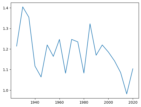
Almost always above 1, but all over the place

are the betas really changing like that or is that sample uncertainty?

Lets report the standard errors for each 2-year period

#here is the first time we use the an anonymous function (lambda)
# A lambda function is an anonymous function defined using the `lambda` keyword.
# It is used to create small, one-line functions without formally defining them using `def`.
# In this case, the lambda function takes a DataFrame `x` as input and performs the following steps:
# 1. Fits an OLS regression model using `x['re']` as the dependent variable and `x['Mkt-RF']` as the independent variable.
# 2. Extracts the standard error of the coefficient for `Mkt-RF` from the fitted model.
# The lambda function is applied to each group created by the `groupby` method.

df.groupby((df.index.year // 2) * 2).apply(lambda x: sm.OLS(x['re'], sm.add_constant(x['Mkt-RF'])).fit().bse['Mkt-RF']).plot()

<Axes: >

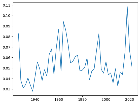
Standard errors are much larger now!

It increase many fold–is that surprising? What do you think is going on?

Might be useful to look at different sampling (30,5,2,1) to get intuition

# lets plot the point estimates and the confidence intervals
y=1 # # you can change this to 5, 10, etc. to change the size of the sample
a=df.groupby((df.index.year // y) * y).apply(lambda x: sm.OLS(x['re'], sm.add_constant(x['Mkt-RF'])).fit().bse['Mkt-RF'])
b=df.groupby((df.index.year // y) * y).apply(lambda x: sm.OLS(x['re'], sm.add_constant(x['Mkt-RF'])).fit().params['Mkt-RF'])
plt.figure(figsize=(10, 6))
plt.plot(b.index, b, label='Coefficient')
plt.fill_between(b.index, b - 1.96 * a, b + 1.96 * a, color='b', alpha=0.2, label='95% Confidence Interval')
plt.xlabel('Year')
plt.ylabel('Coefficient')
plt.title('Coefficient Over Time with 95% Confidence Interval')
plt.legend()
plt.show()

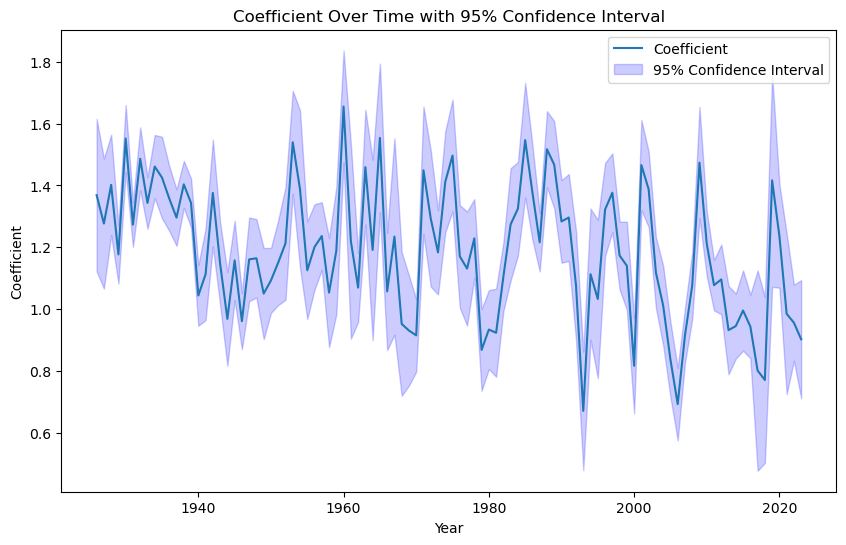
Sometimes standard errors can be deceiving

Our estimation is super confident of the beta on a particular year, but we need to know the beta NEXT year–or at the very least next month if you want to use the beta for hedging for example

b

plt.scatter(b.shift(1), b)
plt.plot(b.shift(1), b.shift(1),'-')

[<matplotlib.lines.Line2D at 0x22aa69f9700>]

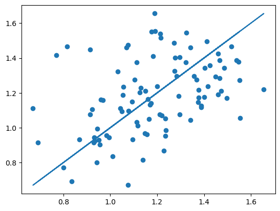
There is a relationship but much more variability then the standard errors suggest

sm.OLS(b[1:], sm.add_constant(b.shift(1)[1:])).fit().summary()

OLS Regression Results

Dep. Variable:	y	R-squared:	0.169
Model:	OLS	Adj. R-squared:	0.161
Method:	Least Squares	F-statistic:	19.36
Date:	Sun, 15 Dec 2024	Prob (F-statistic):	2.83e-05
Time:	00:08:26	Log-Likelihood:	20.745
No. Observations:	97	AIC:	-37.49
Df Residuals:	95	BIC:	-32.34
Df Model:	1
Covariance Type:	nonrobust

	coef	std err	t	P>|t|	[0.025	0.975]
const	0.6919	0.113	6.096	0.000	0.467	0.917
0	0.4137	0.094	4.400	0.000	0.227	0.600

Omnibus:	2.395	Durbin-Watson:	2.029
Prob(Omnibus):	0.302	Jarque-Bera (JB):	2.408
Skew:	0.359	Prob(JB):	0.300
Kurtosis:	2.717	Cond. No.	11.4

Notes:
[1] Standard Errors assume that the covariance matrix of the errors is correctly specified.

How do we interpret these coefficients?

8.2.1. Exponential decay models

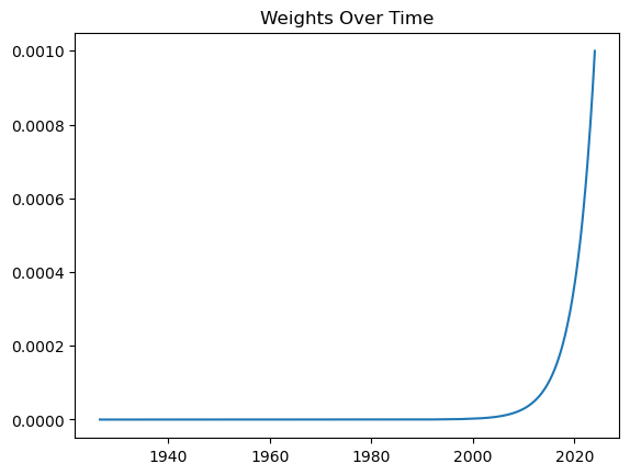
People in the industry also like exponential decay models

Instead of simply ignoring past observations, you instead put less weight on them

Instead of OLS you do GLS with weights given by

\[W_t=\frac{e^{-\delta(T-t)}}{\sum_t^T e^{-\delta(T-t)}}\]

X = df['Mkt-RF']
X = sm.add_constant(X)  # Adds a constant term to the predictor
y = df['re']
n=y.shape[0]
decay_rate = 0.001 # Lambda controls the decay rate

df['weights']= y*0+np.exp(-decay_rate * np.arange(n)[::-1])  # Reverse order for recent weights
df['weights'] /= df['weights'].sum()  # Normalize weights to sum to 1 (optional)

plt.plot(df['weights'])
plt.title('Weights Over Time')

Text(0.5, 1.0, 'Weights Over Time')

model = sm.WLS(y, X, weights=df['weights'])
results = model.fit()

# Display results
print("Regression Summary:")
print(results.summary())

Regression Summary:
                            WLS Regression Results                            
==============================================================================
Dep. Variable:                     re   R-squared:                       0.344
Model:                            WLS   Adj. R-squared:                  0.344
Method:                 Least Squares   F-statistic:                 1.346e+04
Date:                Sun, 15 Dec 2024   Prob (F-statistic):               0.00
Time:                        00:25:21   Log-Likelihood:                -56194.
No. Observations:               25646   AIC:                         1.124e+05
Df Residuals:                   25644   BIC:                         1.124e+05
Df Model:                           1                                         
Covariance Type:            nonrobust                                         
==============================================================================
                 coef    std err          t      P>|t|      [0.025      0.975]
------------------------------------------------------------------------------
const          0.0001      0.000      1.237      0.216   -8.14e-05       0.000
Mkt-RF         1.0609      0.009    116.020      0.000       1.043       1.079
==============================================================================
Omnibus:                    16784.641   Durbin-Watson:                   2.000
Prob(Omnibus):                  0.000   Jarque-Bera (JB):          8449883.622
Skew:                           1.875   Prob(JB):                         0.00
Kurtosis:                      91.845   Cond. No.                         81.3
==============================================================================

Notes:
[1] Standard Errors assume that the covariance matrix of the errors is correctly specified.

8.3. Variances

Variances come in two flavors. Factor variance and idiosyncratic variance.

Both tend to move together at high frequencies (days, weeks, a few months)

At horizons longer than 1 year, you are better off with low frequency estimates of variances–say use a two year-five year sample of daily returns

Fro investment horizons shorten than a month you certainly need to pay attention to higher frequency variation. So you might estimate using 3-month, 1-month , and even one day of data using minute-by-minute data

Lets start with the factor variance, that is the variance of the market

• For intuition I will annualize it. Always look at these moments at yearly frequency so you develop intuition about what to expect and quickly detect if something is wrong

• Because our data is daily, this means multiplying by the number of days in a year

• I will also be taking the square-root and look at standard deviation instead of variance

\[Standard~deviation=\sqrt{Variance}\]

(df['Mkt-RF'].var()*252)**0.5

0.17158032498498688

Volatility is 17% in a year

Does it move around? Look at 5 years, yearly, monthly

# Note: This is the first time we will be using the rolling method

# The rolling method calculates a moving window statistic (e.g., mean, std) over a specified window size.
# Here, it computes the standard deviation of 'Mkt-RF' for the last 'freq' days at each point in time.
# This provides a time series of rolling standard deviations, which is then annualized and plotted.


# Calculate the rolling standard deviation of the 'Mkt-RF' column over a specified window
# The window size is defined by 'freq', which corresponds to 10 years of daily data (252 trading days per year)
# The rolling standard deviation is annualized by multiplying by the square root of 252
# The resulting rolling standard deviation (annualized volatility) is then plotted over time

freq=252*10
(df['Mkt-RF'].rolling(window=freq).std()*252**0.5).plot()

<Axes: >

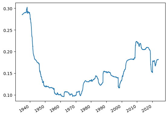
What do you notice?

Clearly the REALIZED VOLATILITY, just like the REALIZED RETURN, moves around a lot

Does that mean that actual forward looking volatility moves around?

Yes! That is Nobel Prize worth insight!

Rob Engle won the nobel prize for developing models that forecast volatility.

[

We will look at volatility forecasting more carefully when we look at volatility timing strategies

Here I will do a simple regression based on the idea that volatility is persistence

We will estimate an AR(1) model

\[RV_{t+1}=a+bRV_t+\epsilon_{t+1}\]

If vol persistent–surely looks like it–b>0 and past vol allow us to forecast future vol

In practice people use very rich models ARCH, GARCH, Multi-frequency AR models, and also data from option markets–for example VIX

We will start by looking at monthly realized variance

• Using daily data for month t, construct the market return “realized variance” during month t

  \[rv_t=\sum_{d \in days~ in ~month ~t}\frac{(r_d- \overline{r})^2}{N_{days}},\]

where \(\overline{r}\) is the average return within the month

# Group the data by month-end dates
# pd.offsets.MonthEnd(0) ensures that the grouping aligns with the month-end of each date
# so all returns in the same month are grouped together
#So I can just compute the variance of this group (say 1/1/2020,1/2/2020,...1/31/2020) will all be 1/31/2020
# For each group, i.e. returns in the same month, calculate the variance of 'Mkt-RF' and annualize it by multiplying by 252

df_var=df.groupby(df.index+pd.offsets.MonthEnd(0)).apply(lambda x:x['Mkt-RF'].var()*252)

# here I am taking the square root of the variance to get the standard deviation (volatility) and plotting it
(df_var**0.5).plot()

---------------------------------------------------------------------------
NameError                                 Traceback (most recent call last)
Cell In[1], line 6
      1 # Group the data by month-end dates
      2 # pd.offsets.MonthEnd(0) ensures that the grouping aligns with the month-end of each date
      3 # so all returns in the same month are grouped together
      4 # For each group, i.e. returns in the same month, calculate the variance of 'Mkt-RF' and annualize it by multiplying by 252
----> 6 df_var=df.groupby(df.index+pd.offsets.MonthEnd(0)).apply(lambda x:x['Mkt-RF'].var()*252)
      8 # here I am taking the square root of the variance to get the standard deviation (volatility) and plotting it
      9 (df_var**0.5).plot()

NameError: name 'df' is not defined

You should see a lot of clustering which suggests you can forecast using past values of variance

import statsmodels.api as sm


# Shift the variance series by one period to create the lagged variable, 
# i.e. using the previous month's variance as a predictor for the current month's variance
# When you shift the series, the first row will be NaN because there is no previous month for the first month
# if you were to use -1 you would be using the next month's variance as a predictor for the current month's variance
# would that make sense? No, because you would be using future information to predict the past
df_var_lag = df_var.shift(1)

# Drop the first row with NaN value
# you have to drop in both series to align them correctly for regression
df_var = df_var[1:]
df_var_lag = df_var_lag[1:]

# Define the independent variable (lagged variance) and add a constant term
X = sm.add_constant(df_var_lag)

# Define the dependent variable (current variance)
y = df_var

# Fit the regression model
model = sm.OLS(y, X).fit()

# Print the summary of the regression
print(model.summary())

                            OLS Regression Results                            
==============================================================================
Dep. Variable:                      y   R-squared:                       0.290
Model:                            OLS   Adj. R-squared:                  0.290
Method:                 Least Squares   F-statistic:                     477.8
Date:                Sun, 15 Dec 2024   Prob (F-statistic):           4.68e-89
Time:                        08:58:31   Log-Likelihood:                 1844.6
No. Observations:                1169   AIC:                            -3685.
Df Residuals:                    1167   BIC:                            -3675.
Df Model:                           1                                         
Covariance Type:            nonrobust                                         
==============================================================================
                 coef    std err          t      P>|t|      [0.025      0.975]
------------------------------------------------------------------------------
const          0.0133      0.002      8.185      0.000       0.010       0.016
0              0.5390      0.025     21.859      0.000       0.491       0.587
==============================================================================
Omnibus:                     1642.358   Durbin-Watson:                   2.049
Prob(Omnibus):                  0.000   Jarque-Bera (JB):           514248.392
Skew:                           7.744   Prob(JB):                         0.00
Kurtosis:                     104.577   Cond. No.                         16.9
==============================================================================

Notes:
[1] Standard Errors assume that the covariance matrix of the errors is correctly specified.

• you see we can forecast quite a bit of variation even with a only using the last month variance

8.3.1. Indio Vol

Lets look now at the idiosyncratic component

Recall that

\[\epsilon=r^e-(\alpha+\beta*f)\]

and

\[Var(\epsilon)=Var(r^e-\beta*f)\]

So the variance of the idio component very much depends on your estimate of beta.

Industry models will make them consistent with each other

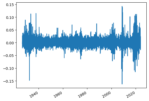
Here we will fix our beta estimate for the whole sample and then look at variation in the volatility of residuals the same we did for the variance of the market

df=df.dropna()
X = df['Mkt-RF']
X = sm.add_constant(X)  # Adds a constant term to the predictor
y = df['re']
model = sm.OLS(y, X).fit(dropna=True)
df['e']=model.resid
df['e'].plot()

<Axes: >

(df['e'].rolling(window=252).std()*252**0.5).plot()
(df['Mkt-RF'].rolling(window=252).std()*252**0.5).plot()
plt.legend(['epsilon','Market Return'])

<matplotlib.legend.Legend at 0x22ab7635e80>

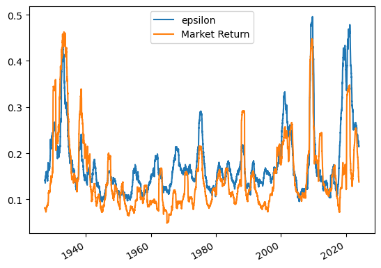
What do you see?

((df.groupby(df.index+pd.offsets.MonthEnd(0))['e'].var()*252)**0.5).plot()
((df.groupby(df.index+pd.offsets.MonthEnd(0))['Mkt-RF'].var()*252)**0.5).plot()

<Axes: >

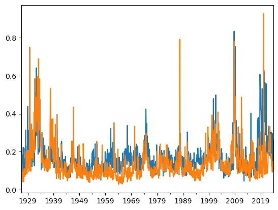
You see a very similar picture

8.3.2. Cross-Section vs Time-series

• Variances tend to move up and down together

• you can repeat the forecasting exercise we did for the market variance to check out degree of variation

• One thing that will be really important is to be able to detect variation in these moments across stocks

• Here we are exploring the extent we can detect variation over time, but lots of trading strategies will be about comparing different stocks and be able to tell which one is more volatile going forward

• By and large the answer for both beta and variance is that we can using reasonable lookback windows

• Typically two years is a good window , but lots of fine tuning around it

8.4. Expected returns

Expected returns have three components

\[E[r]=rf+\alpha + b*E[f]\]

• the risk-free rate–> directly observed in financial markets

• The Factor risk-premia

• The alpha

8.4.1. Factor Risk-Premia

• While conceptually both alpha and risk premia are both expected excess returns, in practice our approach is very different

• Factor risk-premia likely move around, but we think of then as a more stable features of the economic environment

• They are compensation for systematic risk, so they don’t go away just because investors are aware of it

  • Specially true for risk-premia on the market factor

• We are more comfortable in using long data sets to measure it

We will now look at the risk-premia on the market and discuss how to think about the estimation, how to think about the precision of these estimates and briefly discuss how it might move around over time

If We think a risk-premia does not move too much over time, then our best estimate is the sample average of the longest sample we can put our hands on

\[\hat{E}[r^e]=\frac{1}{T}\sum_{t=1}^T r^e_t\]

• If observations are serially uncorrelated over time then the standard deviation of a sample average is simply

\[se(\hat{E}[r^e])=\sqrt{\frac{Var(r^e_t)}{T}}\]

• Returns of most liquid assets are sufficiently close to uncorrelated over time for this assumption to be ok

  • It is also easy enough to adjust for serial correlation which we can easily do using a regression library

• The longer the sample, the higher our precision, the lower the standard errors

• The higher the asset variance, the higher our standard errors, the lower our precision

# Calculate the average for the market
market_average = df['Mkt-RF'].mean()
market_std_dev = df['Mkt-RF'].std()
#number of observations
T=(len(df['Mkt-RF'])
# Calculate the standard error of the average
market_average_std_error = market_std_dev /T ** 0.5)

print(f"Market standard deviation: {market_std_dev}")
print(f"Market Average: {market_average}")
print(f"Standard Error of the Average: {market_average_std_error}")

print(f"t-stat relative to zero null: {(market_average-0)/market_average_std_error}")

Standard Error of the Average: 0.010808544518617085
Market Average: 0.0003018248459798799
Standard Error of the Average: 6.749279240098983e-05
t-stat relative to zero null: 4.471956711861479

This is daily so it looks really ugly. Lets look at annual terms

• The mean is multiplied by 252, because there are 252 days in a year

• Variance is also multiplied by 252, so standard-deviaiton gets multiplied by square root

• The number of observations are divided by 252 because now things are in years

# Calculate the average for the market
market_average = (df['Mkt-RF']*252).mean()
market_std_dev = (df['Mkt-RF']).std()*252**0.5
T=((len(df['Mkt-RF'])/252)
# Calculate the standard error of the average
market_average_std_error = market_std_dev / T** 0.5)

print(f"Market standard deviation: {market_std_dev}")
# Calculate the standard error of the average


print(f"Market Average: {market_average}")
print(f"Standard Error of the Average: {market_average_std_error}")

print(f"t-stat relative to zero null: {(market_average-0)/market_average_std_error}")

Market standard deviation: 0.17158032498498688
Market Average: 0.07605986118692974
Standard Error of the Average: 0.017008183685049437
t-stat relative to zero null: 4.47195671186148

Note that the t-stat is invariant to frequency transformation

This makes the very important point that sampling more frequently does not lead to more precise estimates of the expected return

“only time will tell” could not be any truer for means: Both mean and variance are scaled up by the frequency.

Long sample allow us to be very confident that the market risk-premium is positive on average

We can be fairly confident even that risk-premium is higher than 3%

nullh=0.03
print(f"t-stat relative to {nullh} null: {(market_average-nullh)/market_std_error}")

t-stat relative to 0.03 null: 2.708099938232526

Suppose risk-premium is time-varying but moves kind of slowly

Also lets suppose the variance is constant at the sample mean

How long a sample do I need to be 95% confident that the expected value is higher than the value “x”

I need

\[tstat>F^{-1}(0.95)=1.64\]

\[tstat=\frac{\hat{E}[r^e]-x}{se(\hat{E}[r^e])}>F^{-1}(0.95)=1.64\]

\[tstat=\frac{\hat{E}[r^e]-x}{\sqrt{\frac{Var(r^e_t)}{T}}}>F^{-1}(0.95)=1.64\]

manipulating

\[\sqrt{T}\frac{\hat{E}[r^e]-x}{\sigma(r^e_t)}=1.64\]

\[T=1.64^2*\left(\frac{\hat{E}[r^e]}{\sigma(r^e_t)}-\frac{x}{\sigma(r^e_t)}\right)^{-2}\]

• what is this term \(\frac{\hat{E}[r^e]}{\sigma(r^e_t)}\) called?

• The more confident you want to be, the longer the sample you need

• The more volatile the asset the longer the sample

• The higher the expected value you have for the asset, the shorten the sample

• in the case of x=0 this becomes

\[T=1.64^2*\left(\frac{\hat{E}[r^e]}{\sigma(r^e_t)}\right)^{-2}\]

Suppose we have an asset with similar moments as the market (i.e. same SR)

how long a sample do I expect to need to be confident that the asset has indeed positive mean?

quantile = 0.95
value_at_quantile = norm.ppf(quantile)
sr=market_average/market_std_dev
(sr)**(-2)*value_at_quantile**2

13.76824003316407

What does it tell you about opening a hedge fund?

Lets look at the market spliting it in 15 year periods

y=15
a=df.groupby((df.index.year // y) * y).apply(lambda x: x['Mkt-RF'].mean()/(x['Mkt-RF'].std()/x['Mkt-RF'].count()**0.5))
plt.axhline(y=1.64, color='r', linestyle='--', label='1.64 Threshold')
plt.legend()
a.plot()

<Axes: >

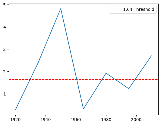
• even then there would be multiple 15 year periods where we would not be 10% sure that the market has a positive expected return

• If you think the market risk-premium moves much faster than this, then the sample mean is fairly unreliable estimator

• This insight will be very important to think about alphas

• This also tells you that timing the market based on past performance–even 15 past performance is a disaster!

Huge literature tries to forecast market return

• They use past volatility (bad, does not work at all)

• Dividend yield (maybe, a bit unreliable)

• earnings yield (similar for dividend yield)

• “Variance-Risk Premium”, basically the VIX minus past vol–that works a bit better, but sample is short, so hard to be sure

IT is very tricky business and even if your model is right

We will look at this in our timing lecture

8.4.2. Alpha is all you need

In one way estimating an alpha is similar to estimating factor risk-premia

• Both are expected values of the excess returns

• Alpha is the expected value of the hedged portfolio

\[\alpha=E[r^e-\beta f]\]

• So you might think the longer the sample, the better right?

• But while for factor premia we have lots of theory telling us that it should move very slowly–it is about aggregate risk–and it should not go away just because people know it

  • it is compensation for aggregate risk!!–people choose not to go all the way because it is risky!

• For alphas, it is the opposite, everyone is jumping when alpha is detected. The whole point is that alpha, real alpha, are premiums that you earn after you HEDGE out any aggregate factor exposure you portfolio have

• What happens with the price as more people buy an asset?

• What happens with the asset actual long-term value?

• What happens with the alpha?

So lets first get a few stocks and compare their alphas. I will focus on one sector

# you probably need to load wrds again if you have been talking for a while :)
conn = wrds.Connection()
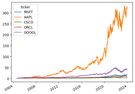
tickers=['MSFT','AAPL','CSCO','ORCL','GOOGL']
df_returns = get_daily_wrds(conn,tickers).dropna()

df_factor = get_factors()
df_return, df_factor = df_returns.align(df_factor, join='inner', axis=0)

df_re=df_return.subtract(df_factor['RF'],axis=0)

print(df_re.head())
(1+df_re).cumprod().plot()

[10104, 10107, 14593, 76076, 90319]

c:\Users\alan.moreira\Anaconda3\lib\site-packages\pandas_datareader\famafrench.py:114: FutureWarning: The argument 'date_parser' is deprecated and will be removed in a future version. Please use 'date_format' instead, or read your data in as 'object' dtype and then call 'to_datetime'.
  df = read_csv(StringIO("Date" + src[start:]), **params)

ticker          MSFT      AAPL      CSCO      ORCL     GOOGL
2004-08-20  0.002900  0.002881 -0.011568 -0.010607  0.079434
2004-08-23  0.004362  0.009041  0.015840 -0.001020  0.010014
2004-08-24 -0.000050  0.027942 -0.010999  0.002863 -0.041458
2004-08-25  0.011330  0.034379  0.018400  0.006726  0.010725
2004-08-26 -0.004043  0.048664 -0.007814 -0.016396  0.017969

<Axes: >

import statsmodels.api as sm

# Define the period length
period_length = 1

# Create a dictionary to store the results
results_dict = {'Ticker': [], 'Period': [], 'Alpha': [], 'Alpha_SE': [], 'Alpha_Tstat': []}

# Loop through each 5-year period
for start_year in range(df_re.index.year.min(), df_re.index.year.max(), period_length):
    end_year = start_year + period_length - 1
    period_label = end_year
    
    # Filter the data for the current period
    period_mask = (df_re.index.year >= start_year) & (df_re.index.year <= end_year)
    df_re_period = df_re[period_mask]
    df_factor_period = df_factor[period_mask]
    
    # Loop through each column in df_re
    for ticker in df_re.columns:
        try:
            y = df_re_period[ticker]
            X = sm.add_constant(df_factor_period['Mkt-RF'])
            
            # Perform the regression
            model = sm.OLS(y, X, missing='drop').fit()
            
            # Store the results
            results_dict['Ticker'].append(ticker)
            results_dict['Period'].append(period_label)
            results_dict['Alpha'].append(model.params['const']*252)
            results_dict['Alpha_SE'].append(model.bse['const']*252)
            results_dict['Alpha_Tstat'].append(model.params['const']/model.bse['const'])
        except:
            pass

# Convert the results dictionary to a DataFrame

results_df = pd.DataFrame(results_dict)

# Display the results
print(results_df)

   Ticker  Period     Alpha  Alpha_SE  Alpha_Tstat
0    MSFT    2004 -0.024613  0.173236    -0.142075
1    AAPL    2004  1.815150  0.695334     2.610472
2    CSCO    2004 -0.452826  0.381418    -1.187216
3    ORCL    2004  0.339126  0.490395     0.691537
4   GOOGL    2004  1.875807  0.880467     2.130469
..    ...     ...       ...       ...          ...
90   MSFT    2022 -0.028199  0.174405    -0.161688
91   AAPL    2022  0.000443  0.170943     0.002591
92   CSCO    2022 -0.062703  0.216968    -0.288997
93   ORCL    2022  0.160281  0.219380     0.730607
94  GOOGL    2022 -0.170152  0.212610    -0.800300

[95 rows x 5 columns]

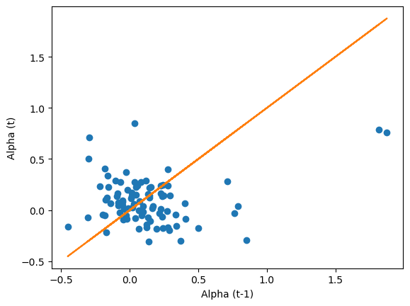
plt.plot(results_df.groupby('Ticker').shift(1)['Alpha'],results_df.Alpha , 'o')
plt.plot(results_df['Alpha'],results_df.Alpha , '-')
plt.xlabel('Alpha (t-1)')
plt.ylabel('Alpha (t)')

Text(0, 0.5, 'Alpha (t)')

plt.plot(results_df.groupby('Ticker').shift(1)['Alpha_Tstat'],results_df.Alpha , 'o')

plt.xlabel('Alpha_Tstat (t-1)')
plt.ylabel('Alpha (t)')

Text(0, 0.5, 'Alpha (t)')

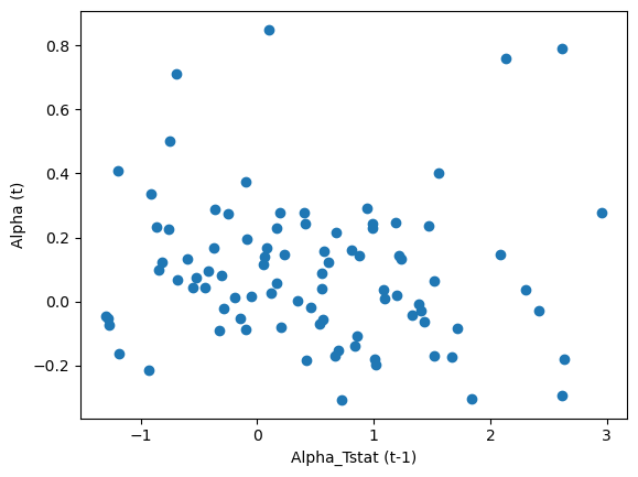
• You see that no matter the horizon there is no PREDICTIVE relationship, last period alpha is not related to future period alpha

• You see that even if you sort on t-stat, it is not better

• Even quite high T-stats are not associated with higher future alphas

• This is not surprising!

• Alpha is all you want and all you need. So everyone is chasing it

• So you expect that alpha of an asset or a trading strategy should be very transient– it will quickly disappears as people learn about it

• This will pose a challenge for you

How do you find alpha?

• Estimating Alpha is hard!

• Every one in the business in searching for alpha

• So true alpha is

  • hard to find

  • disappears quickly

  • if the data was clear, people would already jumped at it

  • Once too much capital is in the trade we say that the trade is “crowded”

  • A Crowded trade can yield NEGATIVE alpha, even if the original idea was right!

  • You have to be right, but also early.

  • If the trade gets crowded after you already in, is that good or bad? What do you do?

If not estimation then what?

You need to think!

• Valuation. You understand a business/market and think the market is not seeing what you are seeing. IT can be short-term insight, like a big client will cancel their services, or long-term prospects for the company business.

  • Warren Buffet whole stick is about this. Read his letters to shareholders. It is all about finding good firms at good value

  • David Einhorn is another example. He famously betted against Leahman Brothers.

  • Often this view will be formed by not only looking at balance sheets , but interacting with company insiders. Even though interactions are public, access allow a good fundamental analyst to see things more clearly (if you get private information, it is of course “easier” but it is illegal and you might end up in jail!)

  • Edge here is having good business judgment. You need to be confident that you are seeing something different form the market and you are right!

  • IT is good discipline to think why people are thinking the wrong thing–you need to understand why the opportunity is there in the first place

• Liquidity provision

  • When firms are downgraded some fund are forced to sell, this often creates reversals

  • Similar effect happens when a firm is dropped from an index, say SP500

  • And it happens in the opposite direction when it is added to the index

  • When mutual fund suffers outflows, they often have to sell, this often creates reversals are as well

  • The bet here is that you understand the reason these buy and sells are happening–and that they are not about fundamental news

  • So you bet the price movements triggered by them will ultimate revert, so you take the other side of the trade–i.e. provide liquidity (at a sweet premium of course)

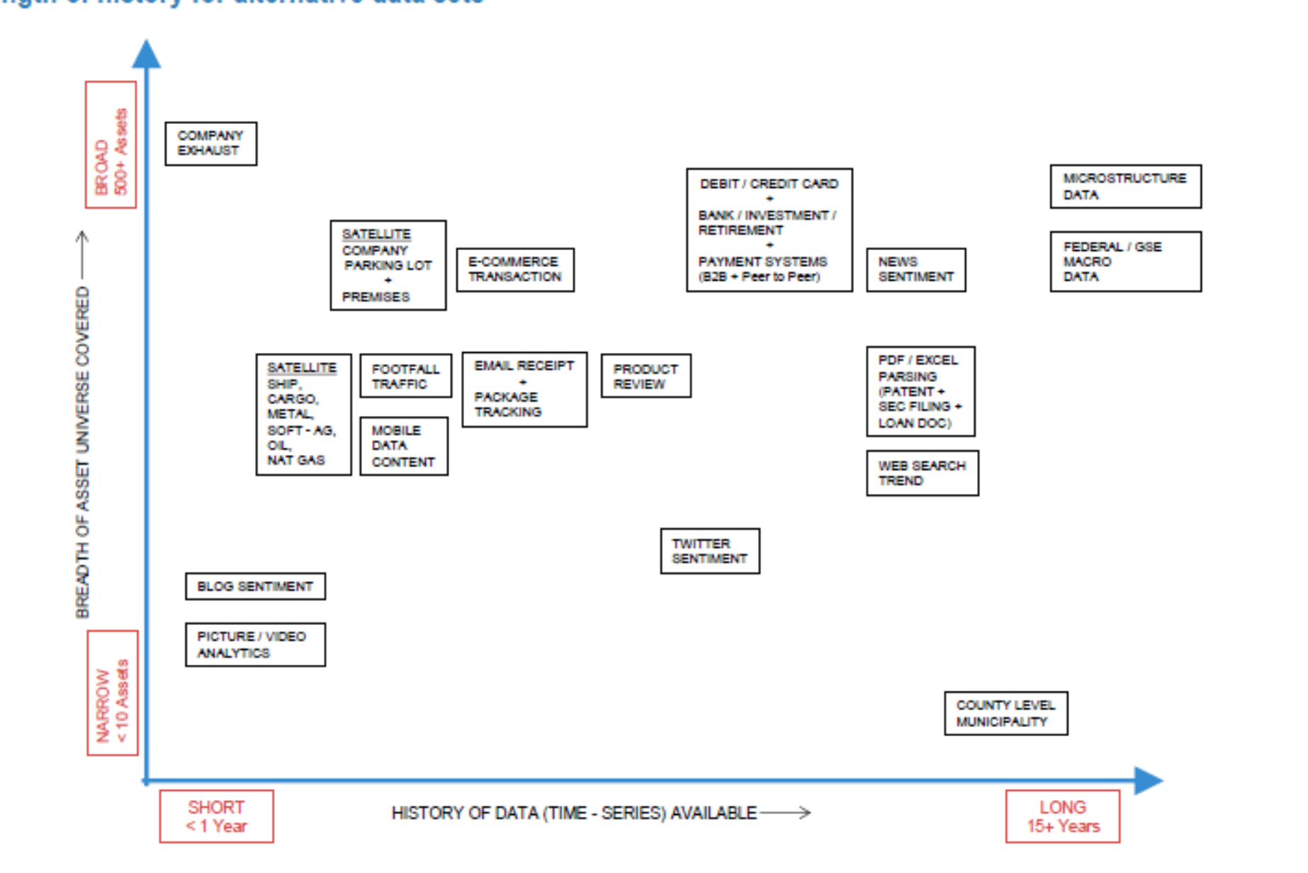
• Data that other people don’t have.

  • Famous example are satellite pictures of parking lots of retail stores–might allow you to predict sales better which hopefully translates into predictions about prices once the market becomes aware of the sales

  • Flow data–this is slightly different from liquidity provision–as you can front run buys/sells if you know that the flows are coming and that they will move markets

  • flooding data, exposure to temperature,

  • supplier data

  • See below a diagram by JP Morgan illustrating the variety of data sources

8.4.2.1. Alpha Quantification Procedure

• Regardless how you get to you alpha, in the end you have to put your trading insights in the same playing field

• Need to choose an horizon, say a month, and put all your alpha in that frequency.

Example:

• Say you have a theory that NVDIA currently trading at 1000 will be at 800 in one year due to things that entirely specific to NVDIA (that is a -20% return)

• Suppose you do not have a theory of when exactly that will happen

• Then you alpha for next month is \((0.8)^{(1/12)}-1\approx-1.8\%\)

• Now suppose you know the timing–so you know this bad news is likely to come only on the last two earnings of the year, then you alpha=0 for the first six months of the year and \((0.8)^{(1/6)}-1\approx-3.6\%\) for last six months of the year

8.4.2.2. Real Alpha is unique and cannot be driven by broad macro factors

• It is useful to develop views for a range of firms/ industries to check that you are not implicitly making a market-wide bet

• if that is your bet, it is silly to hedge market risk–and it is very inefficient to buy a single stock to trade this view

• You should just buy the market in this case!

• And it is important to be aware because it is much harder to be right!

• In practice the notion of “broad macro factors” is much broader then market beta and will often include exposure to a variety of factors, including industry factors

• While it is ok to make a bet on an industry, it is important to know exactly what your trade is

• Buying NVDIA because your bullish on the tech sector is not efficient–you should buy the whole tech sector in that case–much less risk per unit of exposure- as it is not exposed to NVDIA specific factors?

---

📝 Key Takeaways

• Risk parameters are tractable; alpha is the bottleneck. Betas, variances, and even risk-premia can be estimated with historical data, but forecasting alpha requires scarce information or insight.

• Cross-section vs time-series is a trade-off. Cross-sectional snapshots use many assets in one period, while time-series exploits one asset’s history; choose based on data depth and stationarity.

• Sample averages hide regime shifts. Long-run means of factor premia work only if the underlying distribution is stable—watch for structural breaks.

• True alpha decays and crowds out. The moment an idea becomes popular its extra return is competed away, and an overcrowded trade can even turn negative.

• Edge often comes from thinking, not just estimating. Fundamental valuation, understanding forced flows, and leveraging alternative data can reveal mispricings that statistics alone miss.

• Put every idea on the same timeline. Converting a one-year price target into a monthly alpha ensures consistent sizing and portfolio aggregation.

• Test for hidden factor exposure before acting. If the bulk of expected return comes from market or sector movements, a hedged or broader trade is usually superior.

---

Extra Material: The Normal distribution

• Most of what we do does not depend on the assumption of normality

• But normal distributions are very useful in statistical tests

• And they are also not a bad approximation for return data at low frequency (monthly/year)

• Probability that any random draw form a Normal distribution random variable \(\tilde{x}\) is within \(n=1\) standard deviation from the mean is 0.6826

\[Prob(E[\tilde{x}]-1\sigma(\tilde{x})\leq \tilde{x}\leq E[\tilde{x}]+1\sigma(\tilde{x}))=0.6826\]

• \(n=2,Prob(\cdot)=0.9550\)

\[Prob(E[\tilde{x}]-2\sigma(\tilde{x})\leq \tilde{x}\leq E[\tilde{x}]+2\sigma(\tilde{x}))=0.9550\]

• it is convenient to to transform a normally distributed r.v. into units of standard deviations from it’s mean

\[\tilde{z}=\frac{\tilde{x}-E[\tilde{x}]}{\sigma(\tilde{x})}\]

• This follows the “standard” normal distribution, which has mean 0 and and standard deviation 1

• can you show that is indeed the case that z has mean zero and standard devaiton 1?

• This means that the normal distribution is completely characterized by it’s first two moments

• This means that the investment problem is much more tractable too!

• Only two moments to worry about:

  • The expected return of the portfolio

  • it’s variance

  • The probability of really bad tail events will follow immediately from these two!

from scipy.stats import norm

#quantile function
x=norm.ppf(0.95)
print(norm.ppf(0.95))
# cdf
norm.cdf(x)

1.6448536269514722

0.95