Multi-factor models

Collecting wrds
  Downloading wrds-3.4.0-py3-none-any.whl.metadata (5.7 kB)
Collecting packaging<=24.2 (from wrds)
  Downloading packaging-24.2-py3-none-any.whl.metadata (3.2 kB)
Requirement already satisfied: pandas<2.3,>=2.2 in /usr/local/lib/python3.12/dist-packages (from wrds) (2.2.2)
Collecting psycopg2-binary<2.10,>=2.9 (from wrds)
  Downloading psycopg2_binary-2.9.11-cp312-cp312-manylinux2014_x86_64.manylinux_2_17_x86_64.whl.metadata (4.9 kB)
Requirement already satisfied: sqlalchemy<2.1,>=2 in /usr/local/lib/python3.12/dist-packages (from wrds) (2.0.44)
Requirement already satisfied: numpy>=1.26.0 in /usr/local/lib/python3.12/dist-packages (from pandas<2.3,>=2.2->wrds) (2.0.2)
Requirement already satisfied: python-dateutil>=2.8.2 in /usr/local/lib/python3.12/dist-packages (from pandas<2.3,>=2.2->wrds) (2.9.0.post0)
Requirement already satisfied: pytz>=2020.1 in /usr/local/lib/python3.12/dist-packages (from pandas<2.3,>=2.2->wrds) (2025.2)
Requirement already satisfied: tzdata>=2022.7 in /usr/local/lib/python3.12/dist-packages (from pandas<2.3,>=2.2->wrds) (2025.2)
Requirement already satisfied: greenlet>=1 in /usr/local/lib/python3.12/dist-packages (from sqlalchemy<2.1,>=2->wrds) (3.2.4)
Requirement already satisfied: typing-extensions>=4.6.0 in /usr/local/lib/python3.12/dist-packages (from sqlalchemy<2.1,>=2->wrds) (4.15.0)
Requirement already satisfied: six>=1.5 in /usr/local/lib/python3.12/dist-packages (from python-dateutil>=2.8.2->pandas<2.3,>=2.2->wrds) (1.17.0)
Downloading wrds-3.4.0-py3-none-any.whl (14 kB)
Downloading packaging-24.2-py3-none-any.whl (65 kB)
   ━━━━━━━━━━━━━━━━━━━━━━━━━━━━━━━━━━━━━━━━ 65.5/65.5 kB 1.9 MB/s eta 0:00:00
?25hDownloading psycopg2_binary-2.9.11-cp312-cp312-manylinux2014_x86_64.manylinux_2_17_x86_64.whl (4.2 MB)
   ━━━━━━━━━━━━━━━━━━━━━━━━━━━━━━━━━━━━━━━━ 4.2/4.2 MB 18.8 MB/s eta 0:00:00
?25hInstalling collected packages: psycopg2-binary, packaging, wrds
  Attempting uninstall: packaging
    Found existing installation: packaging 25.0
    Uninstalling packaging-25.0:
      Successfully uninstalled packaging-25.0
Successfully installed packaging-24.2 psycopg2-binary-2.9.11 wrds-3.4.0

import wrds

Show code cell content

Hide code cell content

import numpy as np
import pandas as pd
%matplotlib inline
import matplotlib.pyplot as plt
import statsmodels.api as sm

import pandas_datareader.data as web

def get_factors(factors='CAPM',freq='daily'):

    if freq=='monthly':
        freq_label=''
    else:
        freq_label='_'+freq


    if factors=='CAPM':
        fama_french = web.DataReader("F-F_Research_Data_Factors"+freq_label, "famafrench",start="1921-01-01")
        daily_data = fama_french[0]


        df_factor = daily_data[['RF','Mkt-RF']]
    elif factors=='FF3':
        fama_french = web.DataReader("F-F_Research_Data_Factors"+freq_label, "famafrench",start="1921-01-01")
        daily_data = fama_french[0]

        df_factor = daily_data[['RF','Mkt-RF','SMB','HML']]
    elif factors=='FF5':

        fama_french = web.DataReader("F-F_Research_Data_Factors"+freq_label, "famafrench",start="1921-01-01")
        daily_data = fama_french[0]

        df_factor = daily_data[['RF','Mkt-RF','SMB','HML']]
        fama_french2 = web.DataReader("F-F_Research_Data_5_Factors_2x3"+freq_label, "famafrench",start="1921-01-01")
        daily_data2 = fama_french2[0]

        df_factor2 = daily_data2[['RMW','CMA']]
        df_factor=df_factor.merge(df_factor2,on='Date',how='outer')

    else:
        fama_french = web.DataReader("F-F_Research_Data_Factors"+freq_label, "famafrench",start="1921-01-01")
        daily_data = fama_french[0]

        df_factor = daily_data[['RF','Mkt-RF','SMB','HML']]
        fama_french2 = web.DataReader("F-F_Research_Data_5_Factors_2x3"+freq_label, "famafrench",start="1921-01-01")
        daily_data2 = fama_french2[0]

        df_factor2 = daily_data2[['RMW','CMA']]
        df_factor=df_factor.merge(df_factor2,on='Date',how='outer')
        fama_french = web.DataReader("F-F_Momentum_Factor"+freq_label, "famafrench",start="1921-01-01")
        df_factor=df_factor.merge(fama_french[0],on='Date')
        df_factor.columns=['RF','Mkt-RF','SMB','HML','RMW','CMA','MOM']
    if freq=='monthly':
        df_factor.index = pd.to_datetime(df_factor.index.to_timestamp())
    else:
        df_factor.index = pd.to_datetime(df_factor.index)



    return df_factor/100

def get_daily_wrds_multiple_ticker(tickers,conn):

    # Retrieve PERMNOs for the specified tickers
    permnos = conn.get_table(library='crsp', table='stocknames', columns=['permno', 'ticker', 'namedt', 'nameenddt'])
    permnos['nameenddt']=pd.to_datetime(permnos['nameenddt'])
    permnos = permnos[(permnos['ticker'].isin(tickers)) & (permnos['nameenddt']==permnos['nameenddt'].max())]
    # Extract unique PERMNOs
    permno_list = permnos['permno'].unique().tolist()
    print(permno_list)

    # Query daily stock file for the specified PERMNOs
    query = f"""
        SELECT permno, date, ret, retx, prc
        FROM crsp.dsf
        WHERE permno IN ({','.join(map(str, permno_list))})
        ORDER BY date
    """
    daily_returns = conn.raw_sql(query, date_cols=['date'])
    daily_returns = daily_returns.merge(permnos[['permno', 'ticker']], on='permno', how='left')
    # Pivot data to have dates as index and tickers as columns
    daily_returns = daily_returns.pivot(index='date', columns='ticker', values='ret')
    daily_returns=daily_returns[tickers]



    return daily_returns



def get_permnos(tickers,conn):

    # Retrieve PERMNOs for the specified tickers
    permnos = conn.get_table(library='crsp', table='stocknames', columns=['permno', 'ticker', 'namedt', 'nameenddt'])
    permnos['nameenddt']=pd.to_datetime(permnos['nameenddt'])
    permnos = permnos[(permnos['ticker'].isin(tickers)) ]




    return permnos

13. Multi-factor models#

🎯 Learning Objectives

By the end of this chapter, you should be able to:

Understand why investors move beyond CAPM.
Explain how adding multiple systematic factors (size, value, profitability, investment, momentum, etc.) sharpens alpha measurement, improves risk control, and better reflects real‐world return drivers.
Estimate factor betas with a time-series regression.
Learn to regress an asset’s excess returns on a panel of factor returns, interpret coefficients as exposures, and judge statistical reliability.
Translate betas into economic insight through variance decomposition.
Decompose each asset’s total variance into contributions from individual factors and idiosyncratic noise, revealing which risks truly matter.
Build cleaner covariance matrices using a factor structure.
Combine factor loadings with the factor covariance matrix and asset-specific variances to obtain a stable, low-dimensional estimate suitable for portfolio optimization.
Apply multi-factor analysis to real portfolios and ETFs.
Perform step-by-step alpha/beta evaluation of momentum ETFs, ranking funds on both skill (alpha) and risk profile.
Attribute portfolio risk when holdings change.
Project how reallocating capital between strategies alters overall volatility, using factor exposures rather than naïve variance estimates.
Contrast top-down versus bottom-up factor measurement.
Weigh the pros and cons of estimating betas from portfolio returns versus aggregating betas of individual holdings.
Explore the characteristic-based (cross-sectional) alternative.
See how pricing firm-level attributes with cross-sectional regressions yields “characteristic-implied” returns and characteristic-adjusted performance.

So far we have focused on the market as our single factor.

In practice it is standard to use factor models with many factors

Additional factors

soak up risk making measure of alpha easier
Difference out other sources of expected excess returns that are easy to get access to
Allows for better risk management

We deal with this, by simply adding more factors to our model. Say we now have $m$ different factors

\[r_t^i=b_{i,1}f_t^1+b_{i,2}f_t^2+b_{i,3}f_t^3+...+b_{i,m}f_t^m+\epsilon_{i,t}\]

Where $b_{i,j}$ measures the exposure of asset $i$ to factor $j$

IF we stack these exposures in a m by 1 vector $B_i=[b_{i,1},b_{i,2},...b_{i,M}]$ and the factors in a m by 1 vector $F_t=[f^1_t,f^2_t,...,f^m_t]$ we can write this in matrix notation

\[r_t^i=B_i@F_t+u_{i,t}\]

As before we can also stack the individual returns :

\[R_t=B@F_t+U_t\]

where

$R_t$ is a n by 1 vector with the excess returns of the n assets
$B$ is n by m matrix where each row has the exposure of an asset with respect to each M factor and each column has the exposures of the different assets with respect to a particular factor
$U_t$ as before is a n by 1 vector with the residual risk of each asset

“Endogenous” Benchmarking

it is common for large portfolio allocators to set benchmarks for the managers that they allocate to
The most common benchmark is simply returns of the S&P500 which is almost the same thing as the returns of the market portfolio ( large caps dominate the returns of any market-cap portfolio)
You might also have endogenous benchmarks
Use a set of Factors F and estimate $r^b_t=\sum \beta_j F_{j,t}$
I.e use as a bechmark the multifactor combination that best replicates the portfolio.
typically this is not done contractually but implicitly: You will allocate to the different funds based on their alpha
Captures the idea that one should pay different prices for alpha (very hard to get) and beta( easier, the gains are in implementation)

13.1. Estimating a multi-factor model: The Time-series approach#

We start with the factors and estimate the betas using time-series data

This works particularly well when the factors are excess returns themselves

For each asset We run a tim-series regression with the excess returns of the asset as the the dependent variable and the excess returns on the factors as the independent variables

13.2. Application#

What do you get when you invest in a Momentum ETF?

Get daily return data on the larger ETFs claiming to implement the momentum factor
Get factors excess returns: Market, Size (SMB), Value (HML), Profitability (RMW), Investment (CMA) , and Momentum (MOM)
Run a time series regression for each ETF on the factors
Look at alphas and betas

tickers = ["MTUM", "SPMO", "XMMO", "IMTM", "XSMO", "PDP", "JMOM", "DWAS", "VFMO", "XSVM", "QMOM"]
conn=wrds.Connection()
# Get daily returns for the specified tickers
df_ETF=get_daily_wrds_multiple_ticker(tickers,conn)
# Get daily factors
df_factor=get_factors('FF6','daily')
# Align the dataframes
df_ETF, df_factor = df_ETF.align(df_factor, join='inner', axis=0)
# Subtract risk-free rate from ETF returns
df_ETF=df_ETF.subtract(df_factor['RF'],axis=0)

Enter your WRDS username [root]:am16634
Enter your password:··········
WRDS recommends setting up a .pgpass file.
Create .pgpass file now [y/n]?: y
Created .pgpass file successfully.
You can create this file yourself at any time with the create_pgpass_file() function.
Loading library list...
Done
[13512, 13851, 15161, 15725, 17085, 17392, 17622, 90621, 90622, 90623, 91876]

/tmp/ipython-input-1923617899.py:41: FutureWarning: The argument 'date_parser' is deprecated and will be removed in a future version. Please use 'date_format' instead, or read your data in as 'object' dtype and then call 'to_datetime'.
  fama_french = web.DataReader("F-F_Research_Data_Factors"+freq_label, "famafrench",start="1921-01-01")
/tmp/ipython-input-1923617899.py:45: FutureWarning: The argument 'date_parser' is deprecated and will be removed in a future version. Please use 'date_format' instead, or read your data in as 'object' dtype and then call 'to_datetime'.
  fama_french2 = web.DataReader("F-F_Research_Data_5_Factors_2x3"+freq_label, "famafrench",start="1921-01-01")
/tmp/ipython-input-1923617899.py:50: FutureWarning: The argument 'date_parser' is deprecated and will be removed in a future version. Please use 'date_format' instead, or read your data in as 'object' dtype and then call 'to_datetime'.
  fama_french = web.DataReader("F-F_Momentum_Factor"+freq_label, "famafrench",start="1921-01-01")

import statsmodels.api as sm

X = df_factor.drop(columns=['RF'])
X = sm.add_constant(X)  # Adds a constant term to the predictor
y = df_ETF["QMOM"]
X=X[y.isna()==False]
y=y[y.isna()==False]
model = sm.OLS(y, X).fit(dropna=True)
print(model.summary())

                            OLS Regression Results                            
==============================================================================
Dep. Variable:                   QMOM   R-squared:                       0.762
Model:                            OLS   Adj. R-squared:                  0.762
Method:                 Least Squares   F-statistic:                     1217.
Date:                Tue, 18 Nov 2025   Prob (F-statistic):               0.00
Time:                        14:03:26   Log-Likelihood:                 7764.3
No. Observations:                2284   AIC:                        -1.551e+04
Df Residuals:                    2277   BIC:                        -1.547e+04
Df Model:                           6                                         
Covariance Type:            nonrobust                                         
==============================================================================
                 coef    std err          t      P>|t|      [0.025      0.975]
------------------------------------------------------------------------------
const       2.184e-05      0.000      0.129      0.898      -0.000       0.000
Mkt-RF         1.0686      0.016     68.209      0.000       1.038       1.099
SMB            0.4708      0.029     16.161      0.000       0.414       0.528
HML            0.1422      0.025      5.585      0.000       0.092       0.192
RMW           -0.3545      0.037     -9.532      0.000      -0.427      -0.282
CMA           -0.1674      0.046     -3.634      0.000      -0.258      -0.077
MOM            0.5713      0.017     33.671      0.000       0.538       0.605
==============================================================================
Omnibus:                      196.963   Durbin-Watson:                   2.333
Prob(Omnibus):                  0.000   Jarque-Bera (JB):             1241.366
Skew:                           0.004   Prob(JB):                    2.76e-270
Kurtosis:                       6.612   Cond. No.                         292.
==============================================================================

Notes:
[1] Standard Errors assume that the covariance matrix of the errors is correctly specified.

Results=pd.DataFrame([],index=tickers,columns=X.columns)
for ticker in tickers:
    y = df_ETF[ticker]
    X = df_factor.drop(columns=['RF'])
    X = sm.add_constant(X)
    X=X[y.isna()==False]
    y=y[y.isna()==False]
    model = sm.OLS(y, X).fit(dropna=True)
    Results.loc[ticker,:]=model.params
    Results.at[ticker,'t_alpha']=model.tvalues['const']
    Results.at[ticker,'ivol']=model.resid.std()*252**0.5
    Results.at[ticker,'Sample size']=y.shape[0]/252

Results.loc[:,'const']=Results.loc[:,'const']*252
Results.rename(columns={'const':'alpha'},inplace=True)
Results=Results[['alpha','t_alpha','Mkt-RF','SMB','HML','RMW','CMA','MOM','ivol','Sample size']]
Results

	alpha	t_alpha	Mkt-RF	SMB	HML	RMW	CMA	MOM	ivol	Sample size
MTUM	-0.007282	-0.447992	1.024866	-0.105147	-0.057269	-0.127639	-0.027402	0.326001	0.055398	11.690476
SPMO	0.018139	0.771493	1.013642	-0.158997	-0.0495	-0.02651	0.076532	0.255095	0.071108	9.210317
XMMO	0.009412	0.495812	1.040181	0.337055	0.041031	0.030028	-0.106015	0.199402	0.084288	19.805556
IMTM	-0.033995	-1.061967	0.802487	-0.013357	0.056833	-0.132231	0.12593	0.118384	0.100628	9.944444
XSMO	-0.012837	-0.642703	0.98423	0.860196	0.191092	0.100151	-0.092922	0.16577	0.088681	19.805556
PDP	-0.015907	-1.058717	1.054893	0.142871	-0.00844	-0.083458	-0.184182	0.252133	0.063257	17.817460
JMOM	0.004179	0.206044	0.963246	0.012659	-0.064674	-0.07884	-0.066537	0.10529	0.053913	7.123016
DWAS	-0.010497	-0.505913	1.088422	1.076072	0.231479	-0.225859	-0.0794	0.400343	0.072930	12.428571
VFMO	0.011059	0.551059	1.030116	0.449151	0.185205	-0.220818	-0.061642	0.396458	0.052366	6.861111
XSVM	-0.004173	-0.224534	0.932703	0.983764	0.528055	0.329123	0.194403	-0.0564	0.082527	19.805556
QMOM	0.005505	0.128723	1.068629	0.47079	0.142188	-0.354508	-0.167402	0.57135	0.128291	9.063492

How should we evaluate these funds?

Which fund is “better”? Is it all about alpha in this case?

What are other things that we should be looking at?

Is this table providing a fair comparison across funds?

13.3. Performance Attribution#

We can use factor models to decompose a manager strategy
What explains their returns?
What tilts they have? What kind of stocks they like?

13.3.1. Application: What does Cathie Wood Likes ?#

Cathie Wood

Cathie Wood is a renowned stock-picker and the founder of ARK Invest, which manages around 60 billion in assets and invests in innovative technologies such as self-driving cars and genomics. She gained fame for her success in the male-dominated world of investing, her persuasive investment arguments, and her proven track record in the stock market. Prior to founding ARK Invest, she gained experience at The Capital Group, Jennison Associates, and AllianceBernstein, and co-founded Tupelo Capital Management, a hedge fund. Wood is known for her unconventional investment strategies and her advocacy for investing in disruptive technologies, which has garnered her a large following in the investing world. Her estimated net worth is around $250 million.

Citations: https://www.nytimes.com/2021/08/22/business/cathie-wood-ark-stocks.html

df=pd.read_pickle('https://raw.githubusercontent.com/amoreira2/Fin418/main/assets/data/df_WarrenBAndCathieW.pkl')
_temp=df.drop(['BRK'],axis=1).dropna()
# select the columns to use as factors
Factors=_temp.drop(['RF','ARKK'],axis=1)
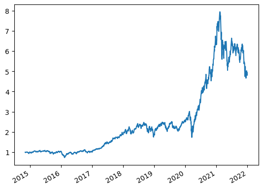
ArK=_temp.ARKK-_temp.RF
(ArK+1).cumprod().plot()
ArK.mean()*252

# _temp=df.drop(['ARKK'],axis=1).dropna()
# # select the columns to use as factors
# Factors=_temp.drop(['RF','BRK'],axis=1)
# BrK=_temp.BRK-_temp.RF
# (BrK+1).cumprod().plot()
# BrK.mean()*252

np.float64(0.2688111096710979)

../../_images/24f53e4a8fc9fb21fc0260800b235920d4dd1f5fa588f0a7503426de5179ddc1.png

What are these factors?

HML is the value strategy that buys high book to market firms and sell low book to market firms
SMB is a size strategy that buys firms with low market capitalization and sell firms with high market capitalizations
RmW is the strategy that buys firms with high gross profitability and sell firms with low gross profitability
CmA is the strategy that buys firms that are investing little (low CAPEX) and sell firms that are investing a lot (high CAPEX)
MOM is the momentum strategy that buy stocks that did well in the last 12 months and short the ones that did poorly

We will discuss more later

for now just think of them as important trading strategies that practicioners know

x= sm.add_constant(Factors*252)
y= ArK*252
results= sm.OLS(y,x).fit()
results.summary()

<Axes: >

../../_images/5d1d5fde74fba087e94e285ff849bbba59640af11e049b0183d8e37562485c16.png

How much can we explain of ARKK return behavior?
What kind of stocks CW likes?
How much of her portfolio variance comes from market exposure alone?
How much comes from being negative value?
If you were to construct a replicating portfolio of her fund what would be the volatility of your residual risk?
Look at the return pattern for the hedged portfolio–when she earned her alpha? Is it smooth? What questions come up?

13.4. Bottom up: from assets factor risk to portfolio factor risk#

Above we estimated fund factor exposures by looking at how the fund co-move with the different factors

An alternative is to look through the fund and compute asset factor loadings and from them compute the fund factor loadings

Consider portfolio with weights $X$ that earns excess returns $r=X@R$ where R is the vector of asset excess returns.

Asset’s excess returns satisfy a factor model

\[R=A+B@F+U\]

then the portfolio satisfies

\[r=X@R=X@(A+B@F+U)=X@A+X@B@F+X@U\]

In scalar notation this is simply

\[r=\sum_i x_i r_i=\sum_i x_i\alpha_i+ \sum_j \sum_i x_i \beta_{i,j}f_j+\sum_i x_i\epsilon_i\]

So the portfolio exposure to factor j is simply the dollar-weighted average of the asset betas

\[\beta_{p,j}=\sum_i x_i \beta_{i,j}\]

For portfolios with high turnover, this approach will lead to better measurement of factor risk
For portfolios that do not trade, then measuring individual asset betas might introduce unnecessary noise and extra work

import pandas as pd

date1='2014-12-31'
date2='2015-12-31'
date3='2016-12-31'
# Define the portfolio data
portfolio_data1 = {
    'date': [date1,date1,date1,date1,date1],
    'ticker': ['AAPL', 'GOOGL', 'MSFT','NVDA','AMZN'],
    'weight': [0.2,0.2, 0.2,0.2,0.2]
}

portfolio_data2 = {
    'date': [date2,date2,date2,date2],
    'ticker': ['COST', 'WMT', 'TGT','KR'],
    'weight': [0.25,0.25, 0.25,0.25]
}
# Concatenate the two dataframes
portfolio_df1 = pd.DataFrame(portfolio_data1)
portfolio_df2 = pd.DataFrame(portfolio_data2)

# Generate monthly dates from date1 to date2 and from date2 to now
date_range1 = pd.date_range(start=date1, end=date2, freq='B')
date_range2 = pd.date_range(start=date2, end=date3, freq='B')

# Create monthly dataframes for each portfolio
monthly_portfolio1 = pd.DataFrame(
    [(date, ticker, weight) for date in date_range1 for ticker, weight in zip(portfolio_df1['ticker'], portfolio_df1['weight'])],
    columns=['date', 'ticker', 'weight']
)
monthly_portfolio2 = pd.DataFrame(
    [(date, ticker, weight) for date in date_range2 for ticker, weight in zip(portfolio_df2['ticker'], portfolio_df2['weight'])],
    columns=['date', 'ticker', 'weight']
)

# Combine the monthly dataframes
final_portfolio_df = pd.concat([monthly_portfolio1, monthly_portfolio2], ignore_index=True)

# import ace_tools as tools
# tools.display_dataframe_to_user(name="Portfolio Monthly Weights", dataframe=final_portfolio_df)

final_portfolio_df

	date	ticker	weight
0	2014-12-31	AAPL	0.20
1	2014-12-31	GOOGL	0.20
2	2014-12-31	MSFT	0.20
3	2014-12-31	NVDA	0.20
4	2014-12-31	AMZN	0.20
...	...	...	...
2353	2016-12-29	KR	0.25
2354	2016-12-30	COST	0.25
2355	2016-12-30	WMT	0.25
2356	2016-12-30	TGT	0.25
2357	2016-12-30	KR	0.25

2358 rows × 3 columns

tickers = final_portfolio_df.ticker.unique().tolist()
#conn=wrds.Connection()
# Get daily returns for the specified tickers
df_stocks=get_daily_wrds_multiple_ticker(tickers,conn)
# Get daily factors
df_factor=get_factors('FF6','daily')
df_factor=df_factor.dropna()
# Align the dataframes

# Subtract risk-free rate from ETF returns
df_stocks=df_stocks.subtract(df_factor['RF'],axis=0)
df_stocks

[10107, 14593, 16678, 49154, 55976, 84788, 86580, 87055, 90319]

ticker	AAPL	GOOGL	MSFT	NVDA	AMZN	COST	WMT	TGT	KR
1928-01-26	NaN	NaN	NaN	NaN	NaN	NaN	NaN	NaN	NaN
1928-01-27	NaN	NaN	NaN	NaN	NaN	NaN	NaN	NaN	NaN
1928-01-28	NaN	NaN	NaN	NaN	NaN	NaN	NaN	NaN	NaN
1928-01-30	NaN	NaN	NaN	NaN	NaN	NaN	NaN	NaN	NaN
1928-01-31	NaN	NaN	NaN	NaN	NaN	NaN	NaN	NaN	NaN
...	...	...	...	...	...	...	...	...	...
2024-11-22	NaN	NaN	NaN	NaN	NaN	NaN	NaN	NaN	NaN
2024-11-25	NaN	NaN	NaN	NaN	NaN	NaN	NaN	NaN	NaN
2024-11-26	NaN	NaN	NaN	NaN	NaN	NaN	NaN	NaN	NaN
2024-11-27	NaN	NaN	NaN	NaN	NaN	NaN	NaN	NaN	NaN
2024-11-29	NaN	NaN	NaN	NaN	NaN	NaN	NaN	NaN	NaN

25409 rows × 9 columns

df=df_stocks.stack()
df.name='eret'
df=final_portfolio_df.merge(df,left_on=['date','ticker'],right_index=True,how='left')
df

	date	ticker	weight	eret
0	2014-12-31	AAPL	0.20	-0.019019
1	2014-12-31	GOOGL	0.20	-0.008631
2	2014-12-31	MSFT	0.20	-0.012123
3	2014-12-31	NVDA	0.20	-0.015710
4	2014-12-31	AMZN	0.20	0.000161
...	...	...	...	...
2353	2016-12-29	KR	0.25	-0.002605
2354	2016-12-30	COST	0.25	-0.006340
2355	2016-12-30	WMT	0.25	-0.002031
2356	2016-12-30	TGT	0.25	-0.005380
2357	2016-12-30	KR	0.25	-0.002323

2358 rows × 4 columns

13.5. TOP DOWN Approach#

For comparison lets estimate this fund factor exposure using the top down approach

Lets construct the portfolio return and then run the multi-factor regression

fund_return=df.groupby('date').apply(lambda x: (x['eret']*x['weight']).sum() )
df_factor, fund_return = df_factor.align(fund_return, join='inner', axis=0)

y=fund_return.copy()
X = df_factor.drop(columns=['RF'])
X = sm.add_constant(X)
X=X[y.isna()==False]
y=y[y.isna()==False]
model = sm.OLS(y, X).fit(dropna=True)
model.summary()

OLS Regression Results
Dep. Variable:	y	R-squared:	0.533
Model:	OLS	Adj. R-squared:	0.527
Method:	Least Squares	F-statistic:	94.64
Date:	Thu, 16 Jan 2025	Prob (F-statistic):	4.66e-79
Time:	17:16:05	Log-Likelihood:	1711.9
No. Observations:	505	AIC:	-3410.
Df Residuals:	498	BIC:	-3380.
Df Model:	6
Covariance Type:	nonrobust

	coef	std err	t	P>\|t\|	[0.025	0.975]
const	0.0005	0.000	1.490	0.137	-0.000	0.001
Mkt-RF	0.9562	0.044	21.531	0.000	0.869	1.043
SMB	-0.1387	0.080	-1.732	0.084	-0.296	0.019
HML	-0.0802	0.097	-0.830	0.407	-0.270	0.109
RMW	0.6811	0.116	5.847	0.000	0.452	0.910
CMA	-0.4294	0.150	-2.855	0.004	-0.725	-0.134
MOM	0.1413	0.050	2.836	0.005	0.043	0.239

Omnibus:	99.867	Durbin-Watson:	1.935
Prob(Omnibus):	0.000	Jarque-Bera (JB):	369.570
Skew:	0.859	Prob(JB):	5.61e-81
Kurtosis:	6.822	Cond. No.	455.

Notes:
[1] Standard Errors assume that the covariance matrix of the errors is correctly specified.

Now suppose you know the time of the portfolio change

I can break the regression, but what do I loose?

    y=fund_return.copy()
    X = df_factor.drop(columns=['RF'])
    y=y[:'2015-12-31']
    X=X[:'2015-12-31']

    X = sm.add_constant(X)
    X=X[y.isna()==False]
    y=y[y.isna()==False]
    model = sm.OLS(y, X).fit(dropna=True)
    display(model.summary())


    y=fund_return.copy()
    X = df_factor.drop(columns=['RF'])
    y=y['2015-12-31':]
    X=X['2015-12-31':]

    X = sm.add_constant(X)
    X=X[y.isna()==False]
    y=y[y.isna()==False]
    model = sm.OLS(y, X).fit(dropna=True)
    model.summary()

OLS Regression Results
Dep. Variable:	y	R-squared:	0.766
Model:	OLS	Adj. R-squared:	0.760
Method:	Least Squares	F-statistic:	134.0
Date:	Thu, 16 Jan 2025	Prob (F-statistic):	1.33e-74
Time:	17:16:07	Log-Likelihood:	905.06
No. Observations:	253	AIC:	-1796.
Df Residuals:	246	BIC:	-1771.
Df Model:	6
Covariance Type:	nonrobust

	coef	std err	t	P>\|t\|	[0.025	0.975]
const	0.0009	0.000	2.041	0.042	3.1e-05	0.002
Mkt-RF	1.0240	0.048	21.290	0.000	0.929	1.119
SMB	-0.2619	0.102	-2.579	0.011	-0.462	-0.062
HML	0.1045	0.129	0.812	0.418	-0.149	0.358
RMW	0.6329	0.168	3.758	0.000	0.301	0.965
CMA	-2.0804	0.229	-9.083	0.000	-2.532	-1.629
MOM	-0.0701	0.063	-1.106	0.270	-0.195	0.055

Omnibus:	88.712	Durbin-Watson:	1.815
Prob(Omnibus):	0.000	Jarque-Bera (JB):	385.398
Skew:	1.374	Prob(JB):	2.05e-84
Kurtosis:	8.386	Cond. No.	576.

Notes:
[1] Standard Errors assume that the covariance matrix of the errors is correctly specified.

OLS Regression Results
Dep. Variable:	y	R-squared:	0.334
Model:	OLS	Adj. R-squared:	0.318
Method:	Least Squares	F-statistic:	20.60
Date:	Thu, 16 Jan 2025	Prob (F-statistic):	1.61e-19
Time:	17:16:07	Log-Likelihood:	870.18
No. Observations:	253	AIC:	-1726.
Df Residuals:	246	BIC:	-1702.
Df Model:	6
Covariance Type:	nonrobust

	coef	std err	t	P>\|t\|	[0.025	0.975]
const	-0.0004	0.001	-0.711	0.478	-0.001	0.001
Mkt-RF	0.7255	0.071	10.272	0.000	0.586	0.865
SMB	0.1198	0.108	1.105	0.270	-0.094	0.333
HML	-0.0642	0.120	-0.536	0.592	-0.300	0.172
RMW	0.7451	0.142	5.230	0.000	0.465	1.026
CMA	0.1497	0.177	0.847	0.398	-0.198	0.498
MOM	0.1587	0.069	2.313	0.022	0.024	0.294

Omnibus:	7.465	Durbin-Watson:	2.104
Prob(Omnibus):	0.024	Jarque-Bera (JB):	12.149
Skew:	-0.092	Prob(JB):	0.00230
Kurtosis:	4.058	Cond. No.	403.

Notes:
[1] Standard Errors assume that the covariance matrix of the errors is correctly specified.

Strategy Abnormal returns

Armed with betas we can construct the fund abnormal returns by simply taking out the part of the performance that is due to factor exposures

\[R_t-\sum_i\beta_i f^i_t\]

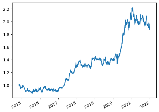
abnormal_return=fund_return-df_factor.drop(columns=['RF'])@model.params[1:]

fund_return.plot()
abnormal_return.plot()

<AxesSubplot:>

../../_images/44e5e2a26830d09d27ce046f734a4c35a58d0ead94749dd24c40efde4a030555.png

How can you produce the abnormal returns more easily simply using outputs from the regression you just run?
Tip: what regression statistic is equal to the average of the abormal return

Bottom UP

Now we estimate the factor loadings for each stock
use our beautiful linear algebra to compute fund exposures

# estimating Factor Betas
df_factor, df_stocks = df_factor.align(df_stocks, join='inner', axis=0)

Xf = df_factor.drop(columns=['RF'])

B=pd.DataFrame([],index=tickers,columns=Xf.columns)
for ticker in df_stocks.columns:
    y = df_stocks[ticker]
    X = sm.add_constant(Xf)
    X=X[y.isna()==False]
    y=y[y.isna()==False]
    model = sm.OLS(y, X).fit(dropna=True)
    B.loc[ticker,:]=model.params[1:]

B

	Mkt-RF	SMB	HML	RMW	CMA	MOM
AAPL	1.030717	-0.107237	-0.008217	0.763479	-1.460115	-0.030158
GOOGL	0.958094	-0.470574	-0.210335	-0.1177	-1.148522	0.144696
MSFT	1.231883	-0.314873	0.077865	0.656917	-1.120852	0.093478
NVDA	1.2523	0.698145	-0.239075	0.321978	-0.472794	0.165622
AMZN	0.995541	-0.438021	0.05142	-0.267262	-2.001092	0.238466
COST	0.791177	-0.035685	0.006976	0.723471	0.02207	0.207055
WMT	0.77975	-0.139923	-0.256882	0.862723	0.496919	0.106942
TGT	0.863384	0.297708	-0.108899	1.244263	0.541671	0.099742
KR	0.740051	0.048948	-0.026441	0.274185	-0.074022	0.309473

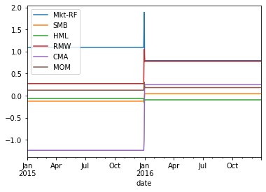
Once we have the Asset betas, then we can compute the fund betas date by date by using the current composition of the portfolio

Obviously this allows you to track the exposure of the fund much better

matters a lot for funds that trade at very high frequency

_temp=final_portfolio_df.merge(B,left_on='ticker',right_index=True,how='left')
Fund_B = _temp.groupby('date').apply(lambda x: pd.Series((x[Xf.columns].values * x['weight'].values.reshape(-1, 1)).sum(axis=0), index=Xf.columns))
Fund_B.plot()
display(Fund_B)

	Mkt-RF	SMB	HML	RMW	CMA	MOM
date
2014-12-31	1.093707	-0.126512	-0.065668	0.271483	-1.240675	0.122421
2015-01-01	1.093707	-0.126512	-0.065668	0.271483	-1.240675	0.122421
2015-01-02	1.093707	-0.126512	-0.065668	0.271483	-1.240675	0.122421
2015-01-05	1.093707	-0.126512	-0.065668	0.271483	-1.240675	0.122421
2015-01-06	1.093707	-0.126512	-0.065668	0.271483	-1.240675	0.122421
...	...	...	...	...	...	...
2016-12-26	0.793590	0.042762	-0.096312	0.776160	0.246659	0.180803
2016-12-27	0.793590	0.042762	-0.096312	0.776160	0.246659	0.180803
2016-12-28	0.793590	0.042762	-0.096312	0.776160	0.246659	0.180803
2016-12-29	0.793590	0.042762	-0.096312	0.776160	0.246659	0.180803
2016-12-30	0.793590	0.042762	-0.096312	0.776160	0.246659	0.180803

523 rows × 6 columns

../../_images/239e144b8036b137251f4eb2d5cd3513b0ca856ee46804c48a032502a2ec91d1.png

How do we estimate the fund abnormal return with this approach?

Note that there is no reason to believe that the asset betas as stable.

As we discussed, there is a lot of thought in deciding which sample is best to estimate the betas

Long samples allow for more precision if the true beta is constant
Shorter samples allow for you to capture time-variation

The general recipe that people use is 1-2 years when using daily data. 5 years when using monthly

13.6. The Cross-Sectional Approach ( or Characteristic-based model)#

In the time-series approach, we start from the factors and estimate the betas

Now we will flip this: we will start from the betas–which are the characteristic–and use a regression to tell us what is the return associated with this characteristic

That is, we will estimate the factors themselves!

The time-series approach requires

factors that are traded
Need to estimate the time-series beta as a first step for abnormal return construction

The Cross-sectional approach goes directly from characteristics to abnormal returns and is often the preferred choice across quant shops because it allows for very large set of factors

The goal is to estimate the returns associated with a characteristic in a particular date, but do that in a way that does not involve the complicated steps of portfolio formation that are hard to do for many characteristics at the same time

Recipe

Get a large set of excess return for stocks (hopefully all) for a given date, R
Get the characteristics of these same stocks , X for this “date”.

Important: the characteristics should be as of the the date before to avoid a spurious regression
it is useful to normalize the characteristics so we can in terms of standard deviations from the average

Run the regression

\[R=BX+\epsilon\]

Note than from the OLS formula–If you have not seen this formula at some point in your life- today is the date!

\[B=(X'X)^{-1}X'R\]

The B coefficients are excess returns themselves as they are just linear combinations of excess returns, i.e. the betas are portfolio returns
They are returns on “pure play” portfolios. Portfolios designed to take a loading of 1 on a charateristic and zero in all the others
$(X'X)^{-1}X'$ are the weights on the pure play portfolio

url = "https://github.com/amoreira2/Fin418/blob/main/assets/data/characteristics_raw.pkl?raw=true"

df_X = pd.read_pickle(url)
# This simply shits the date to be in an end of month basis

df_X.set_index(['date','permno'],inplace=True)
df_X

#df_X.groupby('permno')['re'].std()*12**0.5

		re	rf	rme	size	value	prof	fscore	debtiss	repurch	nissa	...	momrev	valuem	nissm	strev	ivol	betaarb	indrrev	price	age	shvol
date	permno
2006-01-31	10085	0.025224	0.0035	0.0304	14.132980	-0.775040	-2.223152	7	0	1	0.691947	...	0.527791	-0.711504	0.697500	-0.003088	0.003396	1.030378	-0.003491	3.569814	5.480639	0.723779
	10104	0.025984	0.0035	0.0304	18.034086	-2.186115	-0.458025	6	1	1	0.690818	...	0.111133	-1.633254	0.687115	-0.030952	0.012757	1.473739	-0.005108	2.502255	5.480639	1.007820
	10107	0.072982	0.0035	0.0304	19.399144	-1.357207	-1.094087	4	1	1	0.686126	...	0.133546	-1.725634	0.667695	-0.055275	0.006959	1.166726	-0.029431	3.263849	5.480639	0.856907
	10137	0.095710	0.0035	0.0304	15.226304	-0.256102	-2.418484	7	0	0	0.824237	...	0.295023	-0.743060	0.782290	0.137262	0.012228	0.834982	0.124839	3.454738	6.349139	0.952114
	10138	0.057586	0.0035	0.0304	15.913684	-1.553967	-1.227315	7	1	1	0.704786	...	0.213203	-1.661273	0.701101	0.005004	0.006970	1.263471	-0.001327	4.277083	5.476464	0.605547
...	...	...	...	...	...	...	...	...	...	...	...	...	...	...	...	...	...	...	...	...	...	...
2016-12-31	93420	0.011056	0.0003	0.0182	14.337515	1.049163	-2.411521	3	0	1	0.831315	...	-0.433445	-0.202973	0.992891	0.427073	0.036756	1.817194	0.330914	2.706048	4.382027	2.598174
	93422	-0.063881	0.0003	0.0182	15.256946	0.829353	-2.489367	4	1	1	0.857435	...	-0.372774	-0.023505	0.856731	0.223398	0.020980	1.445948	0.127239	2.978586	4.369448	1.555136
	93423	0.039950	0.0003	0.0182	15.502888	-2.128977	-1.246771	6	0	1	0.684617	...	0.123321	-2.341838	0.694344	0.047260	0.013848	0.872411	0.019069	4.054217	4.382027	1.316938
	93429	0.072124	0.0003	0.0182	15.504722	-3.001095	-0.049507	7	1	1	0.683359	...	0.182133	-2.984005	0.686027	0.093973	0.011400	0.738250	-0.054112	4.232656	4.382027	1.210638
	93436	0.127947	0.0003	0.0182	17.262975	-3.328269	-1.793726	2	0	0	0.772211	...	-0.088376	-2.422126	0.763229	-0.042128	0.018539	1.255059	-0.109353	5.243861	4.382027	1.919764

120396 rows × 32 columns

# lets standardize the data
X_std=(df_X.drop(columns=['re','rf','rme']).groupby('date').transform(lambda x: (x-x.mean())/x.std()))

#Lets start by picking a month
date='2006-09'
X=X_std.loc[date]
R=df_X.loc[date,'re']



# Run the regression
# multiplyin by 100 to get percentage
model = sm.OLS(100*R, X).fit()

# Print the summary of the regression
print(model.summary())

                                 OLS Regression Results                                
=======================================================================================
Dep. Variable:                     re   R-squared (uncentered):                   0.158
Model:                            OLS   Adj. R-squared (uncentered):              0.131
Method:                 Least Squares   F-statistic:                              6.017
Date:                Tue, 18 Nov 2025   Prob (F-statistic):                    1.81e-20
Time:                        14:29:41   Log-Likelihood:                         -3128.4
No. Observations:                 962   AIC:                                      6315.
Df Residuals:                     933   BIC:                                      6456.
Df Model:                          29                                                  
Covariance Type:            nonrobust                                                  
==============================================================================
                 coef    std err          t      P>|t|      [0.025      0.975]
------------------------------------------------------------------------------
size           0.3851      0.243      1.585      0.113      -0.092       0.862
value         -2.7649      0.815     -3.392      0.001      -4.364      -1.165
prof           2.2067      0.928      2.377      0.018       0.385       4.028
fscore        -0.1319      0.228     -0.579      0.563      -0.579       0.315
debtiss        0.6979      0.233      3.001      0.003       0.241       1.154
repurch        0.2854      0.231      1.234      0.217      -0.168       0.739
nissa         -0.3563      0.361     -0.987      0.324      -1.065       0.352
growth         0.5318      0.255      2.085      0.037       0.031       1.032
aturnover     -0.2630      1.170     -0.225      0.822      -2.560       2.034
gmargins      -0.2840      0.640     -0.444      0.657      -1.540       0.972
ep            -0.3085      0.263     -1.172      0.242      -0.825       0.208
sgrowth       -0.1833      0.218     -0.842      0.400      -0.611       0.244
lev            3.3657      0.614      5.485      0.000       2.161       4.570
roaa           0.8461      0.327      2.586      0.010       0.204       1.488
roea          -0.3104      0.267     -1.160      0.246      -0.835       0.215
sp            -0.2633      0.401     -0.656      0.512      -1.051       0.525
mom            0.2888      0.384      0.753      0.452      -0.464       1.042
indmom        -1.1630      0.247     -4.706      0.000      -1.648      -0.678
mom12         -0.0708      0.358     -0.198      0.843      -0.773       0.631
momrev        -0.2125      0.230     -0.923      0.356      -0.664       0.239
valuem         1.4420      0.761      1.895      0.058      -0.051       2.935
nissm          0.1557      0.350      0.445      0.657      -0.532       0.843
strev          1.9517      0.585      3.334      0.001       0.803       3.101
ivol          -0.1956      0.318     -0.615      0.539      -0.819       0.428
betaarb        0.4195      0.297      1.412      0.158      -0.163       1.002
indrrev       -2.2913      0.561     -4.084      0.000      -3.392      -1.190
price         -0.2100      0.245     -0.856      0.392      -0.691       0.271
age           -0.4385      0.234     -1.872      0.061      -0.898       0.021
shvol         -0.3185      0.334     -0.955      0.340      -0.973       0.336
==============================================================================
Omnibus:                       52.178   Durbin-Watson:                   1.910
Prob(Omnibus):                  0.000   Jarque-Bera (JB):              137.505
Skew:                          -0.253   Prob(JB):                     1.38e-30
Kurtosis:                       4.782   Cond. No.                         16.9
==============================================================================

Notes:
[1] R² is computed without centering (uncentered) since the model does not contain a constant.
[2] Standard Errors assume that the covariance matrix of the errors is correctly specified.

What this means?

For example this means that a portfolio that takes one “unit” of the the size anomaly and zero of everything else had a return in that month of 0.39%
Value got clobbered with a return of -2.76%
Because we normalize, it means you have a portfolio that has stocks with 1 standard deviation of the characteristic above the characteristic average in that date

What are the portfolios?

#across lines we have the differnt characteristics and across columns we have the different stocks and their wights to implement the portfolio that is exposed to that chracteristic and nothign else

Characteristic_portfolio_weights=np.linalg.inv(X.T@X)@X.T
Characteristic_portfolio_weights.index=X.columns
Characteristic_portfolio_weights

date	2006-09-30
permno	10104	10107	10137	10138	10143	10145	10147	10182	10225	10299	...	89702	89753	89757	89805	89813	90352	90609	90756	91556	92655
size	0.002726	0.004360	-0.000686	-0.000294	-0.001032	0.001538	0.001587	-0.000573	0.000838	-0.000320	...	-0.000651	-0.000082	0.002007	0.000279	0.001528	0.000292	0.000142	-0.000617	-0.000251	0.002837
value	-0.002632	0.006965	0.000676	0.000402	0.001094	0.000918	0.000914	0.001651	0.000402	0.000781	...	0.002959	-0.001872	-0.017175	-0.008553	-0.000069	0.007953	0.001755	-0.002131	-0.004422	-0.000381
prof	-0.004929	-0.005258	0.002034	0.002285	-0.008617	0.002159	-0.000689	-0.001997	0.003331	-0.006068	...	-0.019083	0.002454	0.003818	0.001534	-0.017922	-0.005647	-0.000107	-0.002436	0.000742	0.002495
fscore	-0.000836	0.000893	-0.000555	-0.000177	0.002782	0.001506	0.002053	-0.000181	-0.001518	0.001342	...	0.000608	-0.000435	-0.001723	-0.000495	0.000966	-0.001019	-0.000310	0.001647	-0.000310	-0.000057
debtiss	-0.001236	0.001006	-0.000597	0.000775	-0.000740	0.002011	-0.001833	0.001377	-0.000026	-0.000127	...	0.000919	0.000659	0.001524	-0.000626	-0.001255	-0.000257	0.001134	0.001364	0.001422	-0.000213
repurch	0.000264	-0.001071	0.001303	0.000584	0.002529	0.000491	0.000340	-0.001383	-0.001643	-0.000055	...	-0.000987	-0.001089	-0.002098	-0.001532	0.001370	0.000295	-0.002262	0.001152	0.000432	0.000759
nissa	-0.001617	0.000601	-0.000104	-0.000428	-0.002482	-0.000482	-0.000480	0.000256	-0.001693	0.000070	...	0.001202	0.000048	-0.002312	0.000341	0.000154	0.000719	-0.000753	-0.000134	-0.000160	-0.000975
growth	0.002627	-0.002042	-0.001180	0.000641	0.006734	0.001257	0.000534	0.000382	0.002447	-0.000216	...	-0.000920	-0.000798	0.000595	0.000434	0.001237	-0.000225	0.000504	0.001170	0.000455	0.002122
aturnover	0.004871	0.004464	-0.003664	-0.007132	0.007850	-0.000981	0.000484	-0.008215	-0.003439	0.002336	...	0.023270	-0.004813	-0.000239	-0.002821	0.022379	0.015255	0.000800	0.004665	0.001854	-0.001814
gmargins	0.003855	0.004819	-0.002342	-0.003515	0.005676	-0.002311	0.000605	0.001060	-0.001483	0.003727	...	0.011010	-0.002337	-0.002309	-0.000579	0.010097	0.003309	0.001513	0.000325	-0.000946	-0.002444
ep	0.000271	-0.000069	-0.000293	0.000143	-0.000826	-0.000250	-0.000066	0.006725	0.000147	0.000138	...	-0.000719	0.000504	0.000279	0.000525	-0.000788	-0.011986	0.000181	-0.001006	-0.000486	-0.000425
sgrowth	-0.000287	0.000121	0.000095	-0.000050	0.001933	0.000055	0.000081	-0.000231	-0.000377	0.000371	...	-0.000251	-0.000266	-0.000869	-0.000080	-0.000567	-0.001799	-0.000175	0.000012	0.000174	-0.000431
lev	-0.001423	-0.001301	-0.001663	-0.005339	-0.005967	0.000626	-0.000846	-0.012928	-0.000303	-0.003485	...	0.002164	-0.002672	0.003537	0.000205	0.000187	0.009137	0.002843	0.002029	0.002139	0.000065
roaa	0.001069	0.001812	-0.000686	0.002124	-0.008606	-0.001630	-0.000170	-0.002489	-0.001095	0.002394	...	0.000023	0.000402	0.000735	0.001093	-0.001175	0.002575	0.002885	-0.000064	0.000134	-0.001065
roea	-0.000707	-0.000298	0.000059	-0.000892	0.002531	0.000550	0.000388	0.000520	0.000250	-0.000938	...	0.000191	-0.000201	-0.001692	-0.000749	0.000008	0.000998	-0.000370	-0.000188	-0.000506	0.000377
sp	0.000065	0.000296	-0.000223	0.002129	-0.000102	-0.000631	-0.000166	0.017161	-0.000159	0.001461	...	-0.002150	0.000303	-0.001075	0.000744	-0.001675	-0.011035	-0.000667	-0.001549	-0.001146	-0.000327
mom	0.003275	-0.001444	0.000414	0.000814	0.004850	0.000500	-0.000680	-0.001967	0.001638	0.001538	...	-0.000963	0.006294	0.006965	0.000683	0.000819	-0.003108	-0.005419	-0.001557	-0.001139	-0.002296
indmom	-0.001036	-0.000790	0.001130	-0.000069	-0.000559	0.000744	0.001156	-0.000728	-0.003179	-0.000662	...	-0.000162	0.000246	0.000676	0.000207	-0.000602	0.001851	0.000070	0.001938	-0.000137	-0.000500
mom12	-0.000448	-0.000538	0.000771	0.000531	-0.003858	-0.001458	-0.000226	0.000581	-0.001932	-0.001952	...	-0.000535	-0.002585	-0.002551	0.002501	0.000042	0.001954	0.004019	0.001748	0.001367	0.001481
momrev	-0.000637	-0.000340	0.002424	-0.000383	-0.004906	-0.000384	-0.000023	-0.001467	0.000014	-0.000539	...	0.000848	-0.000252	0.002038	-0.002305	-0.000394	0.000808	-0.000372	-0.000406	-0.001321	0.000021
valuem	0.002454	-0.006450	-0.000259	0.000282	-0.000720	-0.001481	0.000044	-0.000981	-0.000074	-0.000625	...	-0.002613	0.003338	0.017058	0.007713	0.001418	-0.005177	-0.001665	0.001393	0.002914	-0.000042
nissm	0.001268	-0.001002	0.000261	0.000340	0.002121	0.000014	-0.000332	-0.001073	0.001485	-0.000074	...	-0.000455	0.000915	0.001289	0.002882	0.000152	0.001970	-0.001322	-0.000142	-0.000059	0.001160
strev	0.001438	0.000856	0.001983	-0.003842	-0.001651	-0.005159	0.008296	-0.001921	-0.000597	0.003292	...	0.000462	0.001209	0.000576	-0.000857	-0.000587	-0.007146	0.001954	0.002193	-0.002015	0.001781
ivol	-0.000693	-0.000813	-0.000575	-0.000243	-0.000003	-0.000482	0.000029	-0.001962	0.000155	-0.002279	...	-0.001825	0.002788	-0.000676	-0.001814	0.000046	-0.000871	-0.001244	0.000096	-0.001520	0.000576
betaarb	0.001033	-0.001787	-0.000101	0.002654	0.001072	0.002249	0.000876	0.000410	-0.000529	0.001736	...	0.000448	0.001858	0.002971	-0.000773	0.000476	0.002359	-0.000862	-0.000513	-0.000372	-0.002154
indrrev	-0.000593	-0.000945	-0.001676	0.004517	0.003180	0.004748	-0.007188	-0.000257	0.000174	-0.003453	...	-0.000215	0.000768	0.001334	0.001912	0.001349	0.008045	-0.002434	0.000882	0.001426	-0.000810
price	-0.002615	-0.001900	-0.000078	0.000075	0.001128	-0.000128	-0.001855	0.000754	0.001165	0.000277	...	0.001324	0.001663	0.003084	-0.001295	0.000703	-0.002491	-0.003785	0.000367	-0.001120	-0.000556
age	0.000211	-0.000759	0.001319	0.000274	0.002850	0.000730	-0.000111	-0.000180	0.001711	0.000712	...	-0.002721	-0.001921	-0.003869	-0.002800	-0.003422	-0.002200	0.000486	0.000351	-0.000007	-0.000230
shvol	-0.000060	0.001666	0.000600	-0.002817	0.002260	-0.001090	0.000591	-0.000607	-0.000647	0.001927	...	0.000396	-0.000141	-0.000070	-0.000177	-0.001354	-0.000996	0.000648	-0.000197	0.000323	-0.000739

29 rows × 962 columns

What do we do with this?

For a given portfolio I can exactly compute it’s charaterestic-adjusted portfolio returns, if I know the portfolio characteristics
I can also construct a time-series of return for each characteristic, by simply splicing together the regression coefficients of different dates.

Essentially I would run a for loop and get a sequence of betas $[\beta_t,\beta_{t+1},...]$ and these would be the returns on the factors

13.6.1. Constructing Characteristic adjusted returns#

We can get the portfolio characteristics and based on that construct the return implied by these characteristics

We then subtract these characteristic returns from the portfolio returns

It is the equivalent of the “hedged portfolios” that uses the betas to hedge. Here we simply use the characterisitc–instead of makign “factor” neutral we make them characteristic neutral

# Step 1: construct 2 portfolios 1 and 2 ( tech and retail)

portfolio_data1 = {'port': [1,1,1,1,1],
    'ticker': ['AAPL', 'GOOG', 'MSFT','NVDA','AMZN'],
    'weight': [0.2,0.2, 0.2,0.2,0.2]
}

portfolio_data2 = {'port': [2,2,2,2],
    'ticker': ['COST', 'WMT', 'TGT','KR'],
    'weight': [0.25,0.25, 0.25,0.25]
}

portfolio_df1 = pd.DataFrame(portfolio_data1)
portfolio_df2 = pd.DataFrame(portfolio_data2)
portfolio_df = pd.concat([portfolio_df1, portfolio_df2], ignore_index=True)
print(portfolio_df)

   port ticker  weight
   1   AAPL    0.20
   1   GOOG    0.20
   1   MSFT    0.20
   1   NVDA    0.20
   1   AMZN    0.20
   2   COST    0.25
   2    WMT    0.25
   2    TGT    0.25
   2     KR    0.25

# Step 2: Get the permnos associated with these ticker so we can do the matching
# our data has permnos, not tickers
#conn=wrds.Connection()
# get the pemnos for the tickers
permno=get_permnos(portfolio_df.ticker.unique(),conn)

permno['namedt'] = pd.to_datetime(permno['namedt'])
permno['nameenddt'] = pd.to_datetime(permno['nameenddt'])

date='2008-03'
d = pd.to_datetime(date)
# note that sometimes the pernmo changes!
# so we need to get the permnos that are valid at the relevant date
permno_d=permno[(permno['nameenddt']>=d) & (permno['namedt']<=d)]

portfolio_df=portfolio_df.merge(permno_d[['permno','ticker']],on='ticker',how='left')
portfolio_df

	port	ticker	weight	permno
0	1	AAPL	0.20	14593
1	1	GOOG	0.20	90319
2	1	MSFT	0.20	10107
3	1	NVDA	0.20	86580
4	1	AMZN	0.20	84788
5	2	COST	0.25	87055
6	2	WMT	0.25	55976
7	2	TGT	0.25	49154
8	2	KR	0.25	16678

# Step 3: merge our portfolio with our main data set that contains returns and characterisitc
# here we are doign just for one date. Of course you can also do for multiple dates.
#IF the portfolios are fixed that is trivial. If the portfolio is changing , then you should have two identifiers for your
#portfolio in step 1 "port" and "date"


X=X_std.loc[date].reset_index()
port_stocks_X=portfolio_df.merge(X,left_on='permno',right_on='permno',how='left')
port_stocks_X

	port	ticker	weight	permno	date	size	value	prof	fscore	debtiss	...	momrev	valuem	nissm	strev	ivol	betaarb	indrrev	price	age	shvol
0	1	AAPL	0.20	14593	2008-03-31	2.410205	-1.315480	0.455224	-0.091077	1.303219	...	0.575718	-1.421058	0.147848	-0.580727	0.330686	0.752957	-0.868990	1.888114	0.398208	2.904418
1	1	GOOG	0.20	90319	2008-03-31	2.528013	-1.118659	0.564933	-0.091077	1.303219	...	0.755154	-1.005315	0.229125	-1.402481	0.158169	-0.694430	-1.224557	3.959159	-2.339689	1.693268
2	1	MSFT	0.20	10107	2008-03-31	3.257090	-1.363239	0.985259	0.755457	1.303219	...	0.726842	-1.531135	-0.438239	-1.377024	-0.637930	-0.456596	-1.195484	-0.492776	0.105671	-0.399737
3	1	NVDA	0.20	86580	2008-03-31	0.680226	-1.634531	0.817117	0.755457	1.303219	...	1.172971	-0.842731	0.223491	-1.079041	1.603828	2.812533	-1.183732	-0.867861	-1.084778	1.545659
4	1	AMZN	0.20	84788	2008-03-31	1.240524	-3.728875	1.118980	-0.091077	1.303219	...	1.249185	-3.528315	0.034269	-1.451173	0.544068	1.264655	-1.341326	0.854323	-0.858657	1.347997
5	2	COST	0.25	87055	2008-03-31	1.154301	0.138992	0.785716	-0.091077	-0.766462	...	-0.499439	-0.268807	-0.301382	-0.674229	-0.579135	-0.414050	-0.454017	0.791327	0.126212	0.223698
6	2	WMT	0.25	55976	2008-03-31	2.960595	-0.322603	1.029022	-0.937610	-0.766462	...	-0.424544	-0.260600	-0.348921	-0.082608	-1.065065	-0.802397	0.221643	0.444707	0.753804	-1.140483
7	2	TGT	0.25	49154	2008-03-31	1.815796	-0.209013	0.909948	1.601991	-0.766462	...	0.974779	-0.055104	-0.423087	-0.319158	0.450388	0.077535	-0.048508	0.536987	0.871398	0.443988
8	2	KR	0.25	16678	2008-03-31	0.934108	-0.149013	1.326149	0.755457	-0.766462	...	-0.172023	-0.295956	-0.406029	-0.282320	-0.487468	-0.728124	-0.006437	-0.671970	1.220560	-0.344465

9 rows × 34 columns

Now we can compute each portfolio characteristic

# step 4: finally we simply average the characteristics within each portfolio
# we now know how value, momentum, and so on is our portfolio as a funciton of what they hold

X_names=X.drop(columns=['permno','date']).columns
port_X=port_stocks_X.groupby('port').apply(lambda x: x['weight'] @ x[X_names])
port_X

/tmp/ipython-input-939177059.py:5: DeprecationWarning: DataFrameGroupBy.apply operated on the grouping columns. This behavior is deprecated, and in a future version of pandas the grouping columns will be excluded from the operation. Either pass `include_groups=False` to exclude the groupings or explicitly select the grouping columns after groupby to silence this warning.
  port_X=port_stocks_X.groupby('port').apply(lambda x: x['weight'] @ x[X_names])

weight	size	value	prof	fscore	debtiss	repurch	nissa	growth	aturnover	gmargins	...	momrev	valuem	nissm	strev	ivol	betaarb	indrrev	price	age	shvol
port
1	2.023212	-1.832157	0.788303	0.247537	1.303219	0.202595	-0.021355	0.558931	0.525197	0.320116	...	0.895974	-1.665711	0.039299	-1.178089	0.399764	0.735824	-1.162818	1.068192	-0.755849	1.418321
2	1.716200	-0.135409	1.012709	0.332190	-0.766462	0.642131	-0.272052	-0.261772	1.427599	-0.806162	...	-0.030307	-0.220117	-0.369855	-0.339578	-0.420320	-0.466759	-0.071830	0.275263	0.742994	-0.204316

2 rows × 29 columns

We can then compute the portfolio “characteristic-implied” returns and the portfolio characteristic-adjusted return

# Step 5:  estimate the return associated with each characteristic  using the entire investment universe
# we already this step above, but I am repeating here for completeness
# you eould have to repeat this procedure date by data if doign that for multiple dates

X=X_std.loc[date]
R=df_X.loc[date,'re']

# Run the regression
model = sm.OLS(R, X).fit()

R_X=model.params
R_X

	0
size	-0.008685
value	0.010048
prof	0.014476
fscore	-0.000212
debtiss	-0.009435
repurch	0.008764
nissa	0.007878
growth	0.001369
aturnover	-0.026765
gmargins	-0.011491
ep	-0.001229
sgrowth	-0.007586
lev	-0.026462
roaa	-0.008852
roea	0.006974
sp	0.007249
mom	0.005713
indmom	-0.008373
mom12	0.003797
momrev	0.000066
valuem	-0.006634
nissm	-0.005530
strev	0.013887
ivol	-0.007777
betaarb	0.003666
indrrev	-0.011385
price	-0.003223
age	0.004363
shvol	-0.007341

dtype: float64

# Step6: compute the charateteristic implied returns by using the portfolio chanrateristics to compute the portfolio returns
#implied by these characteristics. This the equivalent of $\sum \beta f_{t}^i$, but here port_X are the "betas"
# and R_X and the factors--the returns associated with the charateristic

port_characteristic_returns=port_X[X_names] @R_X
print(port_characteristic_returns)

port
1   -0.027497
2    0.006339
dtype: float64

# step 7: Subtract the charateristic implied return from the portfolio return to obtain the charateristic-adjsuted retrun
# this is the equivalent of $R^{port}_t-\sum \beta f_{t}^i$

# portfolio  raw excess return
_temp=portfolio_df.merge(R.reset_index(),left_on='permno',right_on='permno')
R_port=_temp.groupby('port').apply(lambda x: x['weight']@ x['re'])
display('raw returns')
print(R_port)
display('Characteristic-based returns')
print(port_characteristic_returns)
#  characteristic-adjsuted
Port_characteristic_adjsuted_returns=R_port-port_characteristic_returns
display('Characteristic-adjusted returns')
print(Port_characteristic_adjsuted_returns)

/tmp/ipython-input-2696903702.py:6: DeprecationWarning: DataFrameGroupBy.apply operated on the grouping columns. This behavior is deprecated, and in a future version of pandas the grouping columns will be excluded from the operation. Either pass `include_groups=False` to exclude the groupings or explicitly select the grouping columns after groupby to silence this warning.
  R_port=_temp.groupby('port').apply(lambda x: x['weight']@ x['re'])

'raw returns'

port
1    0.029733
2    0.030074
dtype: float64

'Characteristic-based returns'

port
1   -0.027497
2    0.006339
dtype: float64

'Characteristic-adjusted returns'

port
1    0.057230
2    0.023735
dtype: float64

Why practitioners like this?

You don’t need the time-series betas and all the issues with the size of the sample and how they might move around
All you need is the characteristic at a given date, and that characteristic can move around a lot as we estimate date by date
We used no time-series data at all
You can have very large number of factors: can add sector/industry factors, country factors, currency factors, you name it. Just add to your regression

What are the issues?

The main issue is that ignores covariances, so the characteristic-adjusted portfolios are characteristic neutral but not factor neutral
- For example: a stock might be large but co-move with small stocks and not large stocks, a stock might be classified as retail but co-move with tech
- of course we only care about the characteristics because they describe movement in returns
- But this might or might not be true and we re almost certain that it will be suboptimal
- Now as the number of characteristics grow and they describe returns better and better, this becomes less of an issue
- Consistent with the industry practice of have large set of characteristics (often north of 50-100)
Another issue is that this approach will tend to load on small stocks
- Basically the OLS tries to fit all data points equally and most stocks are tiny
- One fix is to use Weighted-Least Squares where you put more weight on larger firms
- or simply estimate your characteristic returns eliminating the smallest stocks–say focus on the top 20% by market cap

##📝 Key Takeaways

Multi-factor models are the industry work-horse. They capture multiple rewarded risks simultaneously, delivering more realistic benchmarks and richer performance attribution.
Alpha is scarce; beta is plentiful. Time-series regressions on standard factors reveal that most “smart-beta” ETFs provide factor exposure, not out-performance—true skill shows up only in the intercept.
Variance decomposition sharpens intuition. Viewing risk as a weighted blend of factor volatilities highlights which exposures dominate and where diversification gains remain.
Factor-based covariance matrices are stabler and more tractable. Using a handful of factors plus idiosyncratic terms avoids the noise that plagues full empirical covariances, improving minimum-variance and risk-parity constructions.
Risk changes with allocation tilts, not just position size. A small weight shift toward a fund with similar betas barely moves portfolio volatility, while the same shift toward a factor-orthogonal fund can raise risk sharply.
Bottom-up attribution excels for high-turnover managers. Refreshing exposures at the holding level avoids the lag and instability that afflict purely return-based estimates.
Characteristic models broaden the toolkit but ignore covariances. They neutralize portfolios on observed attributes quickly and at scale, yet leave hidden co-movement risks untouched—reminding practitioners that factor and characteristic views are complements, not substitutes.

Multi-factor models

Contents

13. Multi-factor models#

13.1. Estimating a multi-factor model: The Time-series approach#

13.2. Application#

13.3. Performance Attribution#

13.3.1. Application: What does Cathie Wood Likes ?#

13.4. Bottom up: from assets factor risk to portfolio factor risk#

13.5. TOP DOWN Approach#

13.6. The Cross-Sectional Approach ( or Characteristic-based model)#

13.6.1. Constructing Characteristic adjusted returns#