
4.12. Data APIs#
4.12.1. 🎯 Learning Objectives#
By the end of this notebook, you will be able to:
Access macroeconomic data — Using the FRED API
Explore alternative data — Google Trends and real-time stock prices
Download factor data — Ken French’s data library via pandas-datareader
Query institutional databases — WRDS for academic-quality financial data
4.12.2. 📋 Table of Contents#
4.12.3. 🛠️ Setup #
#@title 🛠️ Setup: Run this cell first (click to expand)

# Core libraries
import numpy as np
import pandas as pd
import matplotlib.pyplot as plt
%matplotlib inline

# Set consistent plot style
plt.style.use('seaborn-v0_8-whitegrid')
plt.rcParams['figure.figsize'] = [10, 6]
plt.rcParams['font.size'] = 12

# Suppress warnings for cleaner output
import warnings
warnings.filterwarnings('ignore')

print("✅ Core libraries loaded!")
✅ Core libraries loaded!
4.12.4. FRED API #
4.12.4.1. Federal Reserve Economic Data#
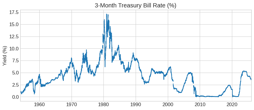
FRED is maintained by the Federal Reserve Bank of St. Louis and contains thousands of macroeconomic and financial time series.
Browse available data: https://fred.stlouisfed.org/categories
Example: 3-Month T-Bill yield: https://fred.stlouisfed.org/series/DTB3
Get your API key: https://research.stlouisfed.org/docs/api/api_key.html
# Install fredapi - a Python wrapper for the FRED API
# This library lets you download economic data directly into pandas DataFrames
!pip install fredapi
Collecting fredapi
  Downloading fredapi-0.5.2-py3-none-any.whl.metadata (5.0 kB)
Requirement already satisfied: pandas in /usr/local/lib/python3.12/dist-packages (from fredapi) (2.2.2)
Requirement already satisfied: numpy>=1.26.0 in /usr/local/lib/python3.12/dist-packages (from pandas->fredapi) (2.0.2)
Requirement already satisfied: python-dateutil>=2.8.2 in /usr/local/lib/python3.12/dist-packages (from pandas->fredapi) (2.9.0.post0)
Requirement already satisfied: pytz>=2020.1 in /usr/local/lib/python3.12/dist-packages (from pandas->fredapi) (2025.2)
Requirement already satisfied: tzdata>=2022.7 in /usr/local/lib/python3.12/dist-packages (from pandas->fredapi) (2025.3)
Requirement already satisfied: six>=1.5 in /usr/local/lib/python3.12/dist-packages (from python-dateutil>=2.8.2->pandas->fredapi) (1.17.0)
Downloading fredapi-0.5.2-py3-none-any.whl (11 kB)
Installing collected packages: fredapi
Successfully installed fredapi-0.5.2
from fredapi import Fred

# Initialize with API key
fred = Fred(api_key='f9207136b3333d7cf92c07273f6f5530')

# Download 3-Month T-Bill rate
tbill_3m = fred.get_series('DTB3')
tbill_3m.plot(title='3-Month Treasury Bill Rate (%)', figsize=(10, 4))
plt.ylabel('Yield (%)')
plt.show()
# Download VIX - the "fear index"
vix = fred.get_series('VIXCLS')
vix.plot(title='VIX Volatility Index', figsize=(10, 4), color='red')
plt.ylabel('VIX')
plt.show()
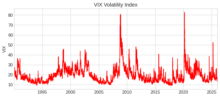
💡 Key Insight:
FRED is your go-to source for macroeconomic data: interest rates, GDP, unemployment, inflation, and more. All free with an API key!
4.12.5. Google Trends #
4.12.5.1. Alternative Data: Search Interest#
Google Trends provides data on search interest over time. This is an example of alternative data — non-traditional data sources that can provide unique insights.
Here I am going to get data from https://serpapi.com/
You can sign up for a free account to get an API_KEY
It allows you to tap all sort of information form Google. Here we will use to get google_trends
Google_trends is often use as a proxy for attention of retail investors
!pip install google-search-results
from serpapi import GoogleSearch
import pandas as pd
import matplotlib.pyplot as plt

# ⚠️ Uncomment the lines below after adding your API Key
#API_KEY='a8667ee3d37e1dd2990c4084515c73d0a53fa6a2bad51fd03afbdcac7a8b9f9d'

# this gives parameters to the API
params = {
  "api_key": API_KEY,
  "engine": "google_trends",
  "q": "GME",
  "date": "all"
}
# This calls the API
search = GoogleSearch(params)
results = search.get_dict()

# now we need to put this in format that is good for plotting

# Extract timeline data from the dictionary and put it dataframe format
timeline = results.get('interest_over_time', {}).get('timeline_data', [])

records = []
for point in timeline:
    row = {'date': point['date']}
    row.update({v['query']: v['extracted_value'] for v in point['values']})
    records.append(row)
df = pd.DataFrame(records)

# Plot

df['date'] = pd.to_datetime(df['date'])
df.set_index('date').plot(title='Google Search Interest: wallstreetbets', figsize=(10, 4))
plt.ylabel('Search Interest (0-100)')
plt.show()
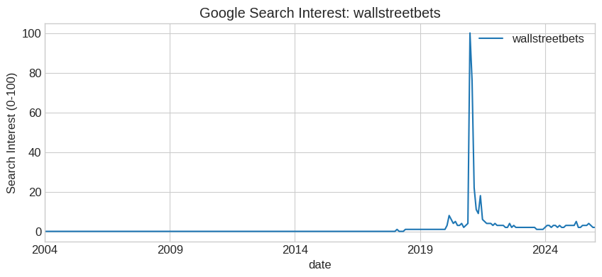
📌 Remember:
Google Trends can signal retail investor interest. The GME spike in early 2021 coincided with the famous “meme stock” rally driven by Reddit.
4.12.6. WallStreet: Real-Time Stock Data #
4.12.6.1. Real-Time Prices and Historical Data#
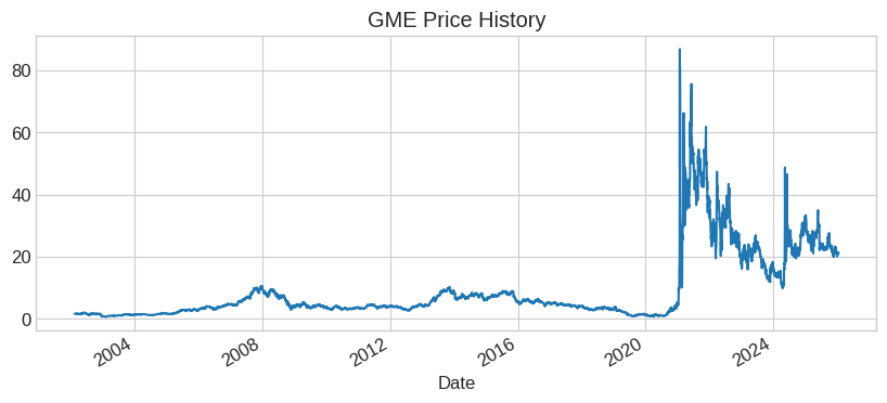
The wallstreet library provides real-time stock quotes and historical data. It also supports options data (calls and puts).
Documentation: mcdallas/wallstreet
# Install wallstreet - real-time stock and options data
# Provides current prices, historical data, and options chains without an API key
!pip install yfinance
Requirement already satisfied: yfinance in /usr/local/lib/python3.12/dist-packages (0.2.66)
Requirement already satisfied: pandas>=1.3.0 in /usr/local/lib/python3.12/dist-packages (from yfinance) (2.2.2)
Requirement already satisfied: numpy>=1.16.5 in /usr/local/lib/python3.12/dist-packages (from yfinance) (2.0.2)
Requirement already satisfied: requests>=2.31 in /usr/local/lib/python3.12/dist-packages (from yfinance) (2.32.4)
Requirement already satisfied: multitasking>=0.0.7 in /usr/local/lib/python3.12/dist-packages (from yfinance) (0.0.12)
Requirement already satisfied: platformdirs>=2.0.0 in /usr/local/lib/python3.12/dist-packages (from yfinance) (4.5.1)
Requirement already satisfied: pytz>=2022.5 in /usr/local/lib/python3.12/dist-packages (from yfinance) (2025.2)
Requirement already satisfied: frozendict>=2.3.4 in /usr/local/lib/python3.12/dist-packages (from yfinance) (2.4.7)
Requirement already satisfied: peewee>=3.16.2 in /usr/local/lib/python3.12/dist-packages (from yfinance) (3.19.0)
Requirement already satisfied: beautifulsoup4>=4.11.1 in /usr/local/lib/python3.12/dist-packages (from yfinance) (4.13.5)
Requirement already satisfied: curl_cffi>=0.7 in /usr/local/lib/python3.12/dist-packages (from yfinance) (0.14.0)
Requirement already satisfied: protobuf>=3.19.0 in /usr/local/lib/python3.12/dist-packages (from yfinance) (5.29.5)
Requirement already satisfied: websockets>=13.0 in /usr/local/lib/python3.12/dist-packages (from yfinance) (15.0.1)
Requirement already satisfied: soupsieve>1.2 in /usr/local/lib/python3.12/dist-packages (from beautifulsoup4>=4.11.1->yfinance) (2.8.1)
Requirement already satisfied: typing-extensions>=4.0.0 in /usr/local/lib/python3.12/dist-packages (from beautifulsoup4>=4.11.1->yfinance) (4.15.0)
Requirement already satisfied: cffi>=1.12.0 in /usr/local/lib/python3.12/dist-packages (from curl_cffi>=0.7->yfinance) (2.0.0)
Requirement already satisfied: certifi>=2024.2.2 in /usr/local/lib/python3.12/dist-packages (from curl_cffi>=0.7->yfinance) (2026.1.4)
Requirement already satisfied: python-dateutil>=2.8.2 in /usr/local/lib/python3.12/dist-packages (from pandas>=1.3.0->yfinance) (2.9.0.post0)
Requirement already satisfied: tzdata>=2022.7 in /usr/local/lib/python3.12/dist-packages (from pandas>=1.3.0->yfinance) (2025.3)
Requirement already satisfied: charset_normalizer<4,>=2 in /usr/local/lib/python3.12/dist-packages (from requests>=2.31->yfinance) (3.4.4)
Requirement already satisfied: idna<4,>=2.5 in /usr/local/lib/python3.12/dist-packages (from requests>=2.31->yfinance) (3.11)
Requirement already satisfied: urllib3<3,>=1.21.1 in /usr/local/lib/python3.12/dist-packages (from requests>=2.31->yfinance) (2.5.0)
Requirement already satisfied: pycparser in /usr/local/lib/python3.12/dist-packages (from cffi>=1.12.0->curl_cffi>=0.7->yfinance) (2.23)
Requirement already satisfied: six>=1.5 in /usr/local/lib/python3.12/dist-packages (from python-dateutil>=2.8.2->pandas>=1.3.0->yfinance) (1.17.0)
import yfinance as yf

# Single stock - current price
gme = yf.Ticker('GME')
print(f"GME current price: ${gme.info['currentPrice']:.2f}")

# Historical data (returns a DataFrame!)
df = gme.history(period='max')  # or '5y', 'max', etc.
print(df.head())

# Quick plot
df['Close'].plot(title='GME Price History', figsize=(10, 4))
GME current price: $21.10
                               Open      High       Low     Close    Volume  \
Date
2002-02-13 00:00:00-05:00  1.620128  1.693350  1.603296  1.691667  76216000
2002-02-14 00:00:00-05:00  1.712707  1.716073  1.670626  1.683250  11021600
2002-02-15 00:00:00-05:00  1.683250  1.687458  1.658001  1.674834   8389600
2002-02-19 00:00:00-05:00  1.666418  1.666418  1.578047  1.607504   7410400
2002-02-20 00:00:00-05:00  1.615920  1.662210  1.603296  1.662210   6892800

                           Dividends  Stock Splits
Date
2002-02-13 00:00:00-05:00        0.0           0.0
2002-02-14 00:00:00-05:00        0.0           0.0
2002-02-15 00:00:00-05:00        0.0           0.0
2002-02-19 00:00:00-05:00        0.0           0.0
2002-02-20 00:00:00-05:00        0.0           0.0
<Axes: title={'center': 'GME Price History'}, xlabel='Date'>
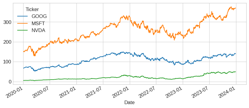
df = yf.download(['NVDA', 'MSFT', 'GOOG'], start='2020-01-01', end='2024-01-01')
df['Close'].plot(figsize=(10, 4))
[*********************100%***********************] 3 of 3 completed
<Axes: xlabel='Date'>
4.12.7. Pandas DataReader: Ken French Library #
4.12.7.1. Academic Factor Data#
Pandas DataReader connects to many data sources. We’re most interested in Ken French’s data library, which provides returns on factor portfolios used in academic finance.
Documentation: https://pandas-datareader.readthedocs.io/en/latest/remote_data.html
# Install pandas-datareader - connects to various financial data sources
# Key feature: access to Ken French's factor data library (297 datasets!)
!pip install pandas_datareader
Requirement already satisfied: pandas_datareader in /usr/local/lib/python3.12/dist-packages (0.10.0)
Requirement already satisfied: lxml in /usr/local/lib/python3.12/dist-packages (from pandas_datareader) (6.0.2)
Requirement already satisfied: pandas>=0.23 in /usr/local/lib/python3.12/dist-packages (from pandas_datareader) (2.2.2)
Requirement already satisfied: requests>=2.19.0 in /usr/local/lib/python3.12/dist-packages (from pandas_datareader) (2.32.4)
Requirement already satisfied: numpy>=1.26.0 in /usr/local/lib/python3.12/dist-packages (from pandas>=0.23->pandas_datareader) (2.0.2)
Requirement already satisfied: python-dateutil>=2.8.2 in /usr/local/lib/python3.12/dist-packages (from pandas>=0.23->pandas_datareader) (2.9.0.post0)
Requirement already satisfied: pytz>=2020.1 in /usr/local/lib/python3.12/dist-packages (from pandas>=0.23->pandas_datareader) (2025.2)
Requirement already satisfied: tzdata>=2022.7 in /usr/local/lib/python3.12/dist-packages (from pandas>=0.23->pandas_datareader) (2025.3)
Requirement already satisfied: charset_normalizer<4,>=2 in /usr/local/lib/python3.12/dist-packages (from requests>=2.19.0->pandas_datareader) (3.4.4)
Requirement already satisfied: idna<4,>=2.5 in /usr/local/lib/python3.12/dist-packages (from requests>=2.19.0->pandas_datareader) (3.11)
Requirement already satisfied: urllib3<3,>=1.21.1 in /usr/local/lib/python3.12/dist-packages (from requests>=2.19.0->pandas_datareader) (2.5.0)
Requirement already satisfied: certifi>=2017.4.17 in /usr/local/lib/python3.12/dist-packages (from requests>=2.19.0->pandas_datareader) (2026.1.4)
Requirement already satisfied: six>=1.5 in /usr/local/lib/python3.12/dist-packages (from python-dateutil>=2.8.2->pandas>=0.23->pandas_datareader) (1.17.0)
from pandas_datareader.famafrench import get_available_datasets

# How many datasets are available?
datasets = get_available_datasets()
print(f"Ken French Library has {len(datasets)} datasets!")
Ken French Library has 297 datasets!
from datetime import datetime
import pandas_datareader.data as web

# Download the 49 Industry Portfolios
start = datetime(1926, 1, 1)
ds = web.DataReader('49_Industry_Portfolios', 'famafrench', start=start)

# See what's included
print(ds['DESCR'])
49 Industry Portfolios
----------------------

This file was created using the 202511 CRSP database. It contains value- and equal-weighted returns for 49 industry portfolios. The portfolios are constructed at the end of June. The annual returns are from January to December. Missing data are indicated by -99.99 or -999. Copyright 2025 Eugene F. Fama and Kenneth R. French

  0 : Average Value Weighted Returns -- Monthly (1193 rows x 49 cols)
  1 : Average Equal Weighted Returns -- Monthly (1193 rows x 49 cols)
  2 : Average Value Weighted Returns -- Annual (98 rows x 49 cols)
  3 : Average Equal Weighted Returns -- Annual (98 rows x 49 cols)
  4 : Number of Firms in Portfolios (1193 rows x 49 cols)
  5 : Average Firm Size (1193 rows x 49 cols)
  6 : Sum of BE / Sum of ME (100 rows x 49 cols)
  7 : Value-Weighted Average of BE/ME (100 rows x 49 cols)
The dataset contains 7 different tables:
Index |
Contents |
|---|---|
0 |
Value-weighted monthly returns |
1 |
Equal-weighted monthly returns |
2 |
Value-weighted annual returns |
… |
… |
6 |
Book-to-market ratios |
# Get value-weighted monthly returns (index 0)
industry_returns = ds[0]
industry_returns.tail()
| Agric | Food | Soda | Beer | Smoke | Toys | Fun | Books | Hshld | Clths | ... | Boxes | Trans | Whlsl | Rtail | Meals | Banks | Insur | RlEst | Fin | Other | |
|---|---|---|---|---|---|---|---|---|---|---|---|---|---|---|---|---|---|---|---|---|---|
| Date | |||||||||||||||||||||
| 2025-07 | -1.94 | -0.38 | -4.12 | 3.38 | -5.84 | 2.04 | -8.73 | -3.33 | -3.10 | 2.51 | ... | -0.42 | -2.06 | 0.14 | 3.11 | -2.51 | 0.82 | -9.74 | 10.67 | 4.49 | -2.32 |
| 2025-08 | 2.81 | 0.13 | 3.43 | 3.49 | 3.87 | 6.39 | 5.00 | 5.69 | 3.27 | 4.25 | ... | 1.99 | 4.21 | 1.54 | 0.85 | 0.88 | 5.11 | 7.49 | 5.79 | -0.20 | 4.46 |
| 2025-09 | -9.46 | -1.77 | -1.54 | -7.12 | -2.09 | -3.06 | -1.69 | 0.91 | -3.54 | -5.42 | ... | -3.89 | 0.49 | 0.80 | -1.06 | -4.61 | 0.13 | 1.63 | -3.50 | 2.96 | -0.75 |
| 2025-10 | -8.64 | -5.43 | 3.16 | 3.37 | -11.53 | 0.73 | -6.36 | -8.03 | -3.04 | -6.04 | ... | -7.86 | -0.24 | 0.02 | 2.85 | -3.60 | -0.10 | -6.36 | -1.88 | -2.97 | -4.21 |
| 2025-11 | 8.12 | 3.14 | 6.20 | 2.36 | 7.82 | 9.20 | -1.53 | 2.25 | 1.14 | 3.88 | ... | 4.45 | 0.55 | 1.77 | -0.42 | 6.60 | 1.35 | 3.30 | 7.15 | 0.29 | 6.18 |
5 rows × 49 columns
# Get book-to-market ratios (index 6)
book_to_market = ds[6]
book_to_market.tail()
| Agric | Food | Soda | Beer | Smoke | Toys | Fun | Books | Hshld | Clths | ... | Boxes | Trans | Whlsl | Rtail | Meals | Banks | Insur | RlEst | Fin | Other | |
|---|---|---|---|---|---|---|---|---|---|---|---|---|---|---|---|---|---|---|---|---|---|
| Date | |||||||||||||||||||||
| 2021 | 0.85 | 0.41 | 0.09 | 0.17 | -0.05 | 0.10 | 0.10 | 0.55 | 0.12 | 0.13 | ... | 0.30 | 0.17 | 0.24 | 0.12 | 0.01 | 0.64 | 0.65 | 0.32 | 0.45 | 0.66 |
| 2022 | 0.71 | 0.39 | 0.10 | 0.18 | -0.05 | 0.20 | 0.11 | 0.50 | 0.11 | 0.13 | ... | 0.32 | 0.17 | 0.21 | 0.11 | 0.02 | 0.53 | 0.51 | 0.29 | 0.36 | 0.63 |
| 2023 | 0.62 | 0.40 | 0.10 | 0.16 | -0.05 | 0.40 | 0.19 | 0.67 | 0.17 | 0.17 | ... | 0.43 | 0.23 | 0.24 | 0.15 | 0.01 | 0.64 | 0.35 | 0.34 | 0.40 | 0.59 |
| 2024 | 0.75 | 0.44 | 0.11 | 0.21 | -0.07 | 0.31 | 0.15 | 0.51 | 0.16 | 0.18 | ... | 0.41 | 0.19 | 0.21 | 0.13 | 0.02 | 0.71 | 0.39 | 0.37 | 0.36 | 0.58 |
| 2025 | 0.60 | 0.48 | 0.10 | 0.24 | -0.05 | 0.31 | 0.10 | 0.44 | 0.15 | 0.22 | ... | 0.35 | 0.20 | 0.19 | 0.11 | 0.01 | 0.57 | 0.38 | 0.32 | 0.31 | 0.58 |
5 rows × 49 columns
4.12.7.2. Browsing All Available Datasets#
# View first 20 available datasets
print("First 20 Ken French datasets:")
for i, name in enumerate(datasets[:20]):
    print(f"  {i+1}. {name}")
First 20 Ken French datasets:
  1. F-F_Research_Data_Factors
  2. F-F_Research_Data_Factors_weekly
  3. F-F_Research_Data_Factors_daily
  4. F-F_Research_Data_5_Factors_2x3
  5. F-F_Research_Data_5_Factors_2x3_daily
  6. Portfolios_Formed_on_ME
  7. Portfolios_Formed_on_ME_Wout_Div
  8. Portfolios_Formed_on_ME_Daily
  9. Portfolios_Formed_on_BE-ME
  10. Portfolios_Formed_on_BE-ME_Wout_Div
  11. Portfolios_Formed_on_BE-ME_Daily
  12. Portfolios_Formed_on_OP
  13. Portfolios_Formed_on_OP_Wout_Div
  14. Portfolios_Formed_on_OP_Daily
  15. Portfolios_Formed_on_INV
  16. Portfolios_Formed_on_INV_Wout_Div
  17. Portfolios_Formed_on_INV_Daily
  18. 6_Portfolios_2x3
  19. 6_Portfolios_2x3_Wout_Div
  20. 6_Portfolios_2x3_weekly
💡 Key Insight:
Ken French’s library is the gold standard for factor research. It includes Fama-French factors, momentum, industry portfolios, and more.
4.12.8. WRDS: Academic Financial Data #
4.12.8.1. The Gold Standard for Research#
WRDS (Wharton Research Data Services) is the premier source for academic financial data. It includes:
CRSP: Stock prices, returns, and market data
Compustat: Balance sheet and income statement data
IBES: Analyst forecasts
And much more…
Register for an account: https://wrds-www.wharton.upenn.edu/register/
# Install WRDS library - official Python interface for WRDS database
# Requires a WRDS account (free for academic users)
!pip install wrds
Collecting wrds
  Downloading wrds-3.4.0-py3-none-any.whl.metadata (5.7 kB)
Collecting packaging<=24.2 (from wrds)
  Downloading packaging-24.2-py3-none-any.whl.metadata (3.2 kB)
Requirement already satisfied: pandas<2.3,>=2.2 in /usr/local/lib/python3.12/dist-packages (from wrds) (2.2.2)
Collecting psycopg2-binary<2.10,>=2.9 (from wrds)
  Downloading psycopg2_binary-2.9.11-cp312-cp312-manylinux2014_x86_64.manylinux_2_17_x86_64.whl.metadata (4.9 kB)
Requirement already satisfied: sqlalchemy<2.1,>=2 in /usr/local/lib/python3.12/dist-packages (from wrds) (2.0.45)
Requirement already satisfied: numpy>=1.26.0 in /usr/local/lib/python3.12/dist-packages (from pandas<2.3,>=2.2->wrds) (2.0.2)
Requirement already satisfied: python-dateutil>=2.8.2 in /usr/local/lib/python3.12/dist-packages (from pandas<2.3,>=2.2->wrds) (2.9.0.post0)
Requirement already satisfied: pytz>=2020.1 in /usr/local/lib/python3.12/dist-packages (from pandas<2.3,>=2.2->wrds) (2025.2)
Requirement already satisfied: tzdata>=2022.7 in /usr/local/lib/python3.12/dist-packages (from pandas<2.3,>=2.2->wrds) (2025.3)
Requirement already satisfied: greenlet>=1 in /usr/local/lib/python3.12/dist-packages (from sqlalchemy<2.1,>=2->wrds) (3.3.0)
Requirement already satisfied: typing-extensions>=4.6.0 in /usr/local/lib/python3.12/dist-packages (from sqlalchemy<2.1,>=2->wrds) (4.15.0)
Requirement already satisfied: six>=1.5 in /usr/local/lib/python3.12/dist-packages (from python-dateutil>=2.8.2->pandas<2.3,>=2.2->wrds) (1.17.0)
Downloading wrds-3.4.0-py3-none-any.whl (14 kB)
Downloading packaging-24.2-py3-none-any.whl (65 kB)
   ━━━━━━━━━━━━━━━━━━━━━━━━━━━━━━━━━━━━━━━━ 65.5/65.5 kB 5.4 MB/s eta 0:00:00
?25hDownloading psycopg2_binary-2.9.11-cp312-cp312-manylinux2014_x86_64.manylinux_2_17_x86_64.whl (4.2 MB)
   ━━━━━━━━━━━━━━━━━━━━━━━━━━━━━━━━━━━━━━━━ 4.2/4.2 MB 57.4 MB/s eta 0:00:00
?25hInstalling collected packages: psycopg2-binary, packaging, wrds
  Attempting uninstall: packaging
    Found existing installation: packaging 25.0
    Uninstalling packaging-25.0:
      Successfully uninstalled packaging-25.0
Successfully installed packaging-24.2 psycopg2-binary-2.9.11 wrds-3.4.0
import wrds
import psycopg2

# Connect to WRDS (will prompt for username/password)
conn = wrds.Connection()
Enter your WRDS username [root]:am16634
Enter your password:··········
WRDS recommends setting up a .pgpass file.
Create .pgpass file now [y/n]?: y
Created .pgpass file successfully.
You can create this file yourself at any time with the create_pgpass_file() function.
Loading library list...
Done
4.12.8.2. Downloading Stock Returns#
WRDS uses SQL queries to access data. Here’s a function to download daily returns for a given stock:
def get_returns(tickers, conn, startdate, enddate):
    """Download daily returns for a list of tickers from WRDS CRSP."""
    ticker = tickers[0]
    df = conn.raw_sql("""
        select a.permno, b.ticker, a.date, a.ret
        from crsp.dsf as a
        left join crsp.msenames as b
        on a.permno=b.permno
        and b.namedt<=a.date
        and a.date<=b.nameendt
        where a.date between '""" + startdate + """' and '""" + enddate + """'
        and b.ticker='""" + ticker + "'")

    df.set_index(['date', 'permno'], inplace=True)
    df = df['ret'].unstack()
    return df
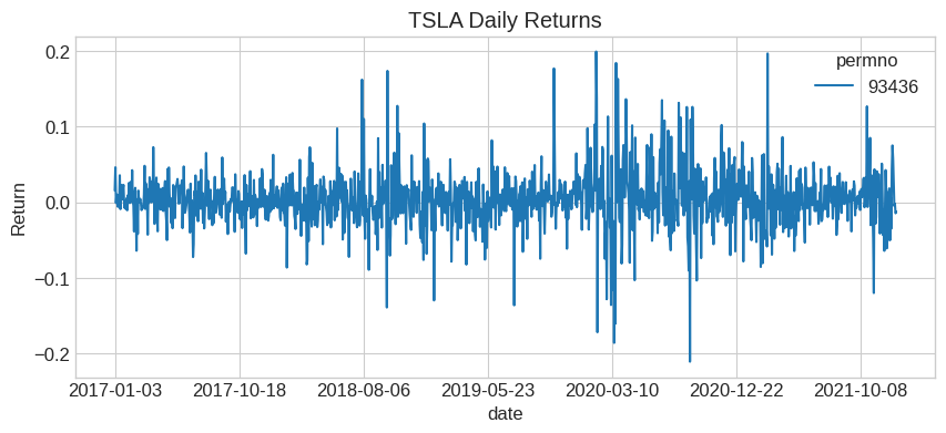
# Download Tesla returns
df_tsla = get_returns(['TSLA'], conn, '1/1/2017', '1/1/2022')
df_tsla.plot(title='TSLA Daily Returns', figsize=(10, 4))
plt.ylabel('Return')
plt.show()
4.12.8.3. Getting Price and Shares Outstanding#
def get_data(tickers, conn, startdate, enddate):
    """Download price and shares outstanding from WRDS CRSP."""
    ticker = tickers[0]
    df = conn.raw_sql("""
        select a.permno, b.ticker, a.date, a.prc, a.shrout
        from crsp.dsf as a
        left join crsp.msenames as b
        on a.permno=b.permno
        and b.namedt<=a.date
        and a.date<=b.nameendt
        where a.date between '""" + startdate + """' and '""" + enddate + """'
        and b.ticker='""" + ticker + "'")

    df.set_index(['date', 'permno'], inplace=True)
    return df
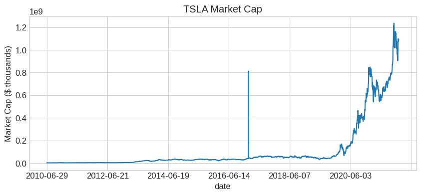
# Download Tesla price data
df = get_data(['TSLA'], conn, '1/1/2005', '1/1/2022')

# Compute market cap (price uses absolute value because negative = bid-ask midpoint)
df['mcap'] = df['prc'].abs() * df['shrout']

# Clean up index and plot
df = df.reset_index().set_index('date')
df['mcap'].plot(title='TSLA Market Cap', figsize=(10, 4))
plt.ylabel('Market Cap ($ thousands)')
plt.show()
📌 Remember:
WRDS variables in CRSP:
ret: daily return (with dividends)
prc: price (negative = bid-ask midpoint). When there was not trade at closing–zero probability for Tesla or any large cap
shrout: shares outstanding (thousands)
vol: trading volume (shares)
4.12.9. 📝 Exercises #
4.12.9.1. Exercise 1: Warm-up — Explore FRED#
🔧 Exercise:
Use the FRED API to:
Download the 10-Year Treasury yield (
GS10)Download the unemployment rate (
UNRATE)Plot both series on the same figure (use two y-axes)
What pattern do you observe during recessions?
# Your code here
💡 Click to see solution
# Download data
gs10 = fred.get_series('GS10')
unrate = fred.get_series('UNRATE')

# Plot with two y-axes
fig, ax1 = plt.subplots(figsize=(12, 5))

ax1.plot(gs10.index, gs10, color='blue', label='10-Year Treasury')
ax1.set_ylabel('10Y Yield (%)', color='blue')

ax2 = ax1.twinx()
ax2.plot(unrate.index, unrate, color='red', label='Unemployment')
ax2.set_ylabel('Unemployment Rate (%)', color='red')

plt.title('Interest Rates vs. Unemployment')
plt.show()

# During recessions: unemployment spikes, rates often fall
4.12.9.2. Exercise 2: Extension — Ken French Factor Data#
🤔 Think and Code:
Download the Fama-French 3-Factor data:
Use
web.DataReader('F-F_Research_Data_Factors', 'famafrench')Extract the monthly factors (index 0)
Plot cumulative returns of MKT-RF, SMB, and HML since 1926
Which factor had the highest cumulative return? Which had the most volatility?
# Your code here
💡 Click to see solution
# Download Fama-French factors
ff = web.DataReader('F-F_Research_Data_Factors', 'famafrench', start=datetime(1926,1,1))
factors = ff[0] / 100  # Convert from percentage to decimal

# Compute cumulative returns
cum_returns = (1 + factors[['Mkt-RF', 'SMB', 'HML']]).cumprod()

# Plot
cum_returns.plot(figsize=(12, 6), title='Cumulative Factor Returns Since 1926')
plt.ylabel('Cumulative Return ($1 initial)')
plt.yscale('log')
plt.legend(['Market-RF', 'Small-Big', 'High-Low B/M'])
plt.show()

# Summary statistics
print("Annualized Statistics:")
print(f"MKT-RF: mean={factors['Mkt-RF'].mean()*12:.2%}, std={factors['Mkt-RF'].std()*np.sqrt(12):.2%}")
print(f"SMB: mean={factors['SMB'].mean()*12:.2%}, std={factors['SMB'].std()*np.sqrt(12):.2%}")
print(f"HML: mean={factors['HML'].mean()*12:.2%}, std={factors['HML'].std()*np.sqrt(12):.2%}")
4.12.9.3. Exercise 3: Open-ended — Industry Analysis#
🤔 Think and Code:
Using the 49 Industry Portfolios:
Compute the annualized mean and volatility for each industry
Create a scatter plot of mean vs. volatility (each point = one industry)
Which industries have the best risk-adjusted returns (highest Sharpe)?
Which industries are the most volatile?
# Your code here
💡 Click to see solution
# Get industry returns (already loaded as ds[0])
ind_ret = ds[0] / 100  # Convert to decimal

# Compute annualized statistics
ind_mean = ind_ret.mean() * 12
ind_std = ind_ret.std() * np.sqrt(12)
ind_sharpe = ind_mean / ind_std

# Scatter plot
fig, ax = plt.subplots(figsize=(10, 8))
ax.scatter(ind_std, ind_mean, alpha=0.7)

# Label each point
for i, ind in enumerate(ind_ret.columns):
    ax.annotate(ind, (ind_std[ind], ind_mean[ind]), fontsize=8)

ax.set_xlabel('Annualized Volatility')
ax.set_ylabel('Annualized Mean Return')
ax.set_title('Industry Risk-Return Tradeoff')
plt.show()

# Top 5 by Sharpe
print("Top 5 industries by Sharpe Ratio:")
print(ind_sharpe.nlargest(5))
4.12.10. 🧠 Key Takeaways #
FRED — Free macroeconomic data (rates, GDP, unemployment) via
fredapiGoogle Trends — Alternative data on search interest via
pytrendsWallStreet — Real-time stock/options quotes via
wallstreetKen French Library — 297 factor/portfolio datasets via
pandas-datareaderWRDS — Academic-quality financial data (requires registration)