
4. Introduction to Asset Returns#
4.1. 🎯 Learning Objectives#
By the end of this notebook, you will be able to:
Define and compute total returns — From prices and dividends
Distinguish returns from excess returns — And explain why it matters
Interpret risk premiums — As compensation for bearing risk
Apply proper data transformations — Merge, clean, and resample return data
4.2. 📋 Table of Contents#
4.3. 🛠️ Setup #
#@title 🛠️ Setup: Run this cell first (click to expand)

# Core libraries
import numpy as np
import pandas as pd
import matplotlib.pyplot as plt
%matplotlib inline

# Set consistent plot style
plt.style.use('seaborn-v0_8-whitegrid')
plt.rcParams['figure.figsize'] = [10, 6]
plt.rcParams['font.size'] = 12

# Suppress warnings for cleaner output
import warnings
warnings.filterwarnings('ignore')

print("✅ Libraries loaded successfully!")
✅ Libraries loaded successfully!
4.4. What is a Stock Return? #
4.4.1. The Core Question#
Imagine you buy a stock today for $100.
Tomorrow it could be worth \(105** or **\)95 or any other value.
How do we measure this change in a standardized way?
4.4.2. The Return Formula#
Total return measures percentage change including dividends:
Where:
\(P_t\) = Price at end of period \(t\)
\(D_t\) = Dividend paid during period \(t\)
\(P_{t-1}\) = Price at start of period
💡 Key Insight:
Returns, not prices, are the fundamental building block of finance. We use returns because they:
Are scale-free (comparable across stocks)
Aggregate naturally over time
Have better statistical properties
4.4.3. Example: Computing Returns from Data#
Let’s load real stock data and compute returns. We’ll use UnitedHealth (UNH).
# Load UNH stock data
url = 'https://raw.githubusercontent.com/amoreira2/UG54/main/assets/data/UNH_data.csv'
df = pd.read_csv(url, parse_dates=['date'], index_col='date')

# Preview the data
print(f"Data range: {df.index.min().date()} to {df.index.max().date()}")
print(f"Columns: {list(df.columns)}")
df.head()
Data range: 1984-10-18 to 2024-12-31
Columns: ['P', 'D']
| P | D | |
|---|---|---|
| date | ||
| 1984-10-18 | 4.8750 | 0.0 |
| 1984-10-19 | 4.6875 | 0.0 |
| 1984-10-22 | 4.6875 | 0.0 |
| 1984-10-23 | 4.5625 | 0.0 |
| 1984-10-24 | 4.6875 | 0.0 |
The data contains:
P: Adjusted closing priceD: Dividend (0 on non-dividend days)
# Compute total return using the formula
df['ret'] = (df['P'] + df['D'] - df['P'].shift(1)) / df['P'].shift(1)

# Display first few rows with the new column
df[['P', 'D', 'ret']].head(10)
| P | D | ret | |
|---|---|---|---|
| date | |||
| 1984-10-18 | 4.8750 | 0.0 | NaN |
| 1984-10-19 | 4.6875 | 0.0 | -0.038462 |
| 1984-10-22 | 4.6875 | 0.0 | 0.000000 |
| 1984-10-23 | 4.5625 | 0.0 | -0.026667 |
| 1984-10-24 | 4.6875 | 0.0 | 0.027397 |
| 1984-10-25 | 4.6250 | 0.0 | -0.013333 |
| 1984-10-26 | 4.5625 | 0.0 | -0.013514 |
| 1984-10-29 | 4.5625 | 0.0 | 0.000000 |
| 1984-10-30 | 4.6250 | 0.0 | 0.013699 |
| 1984-10-31 | 4.6875 | 0.0 | 0.013514 |
📌 Remember:
The first observation is always
NaNbecause we need a prior price. This is expected—we lose one observation when computing returns.
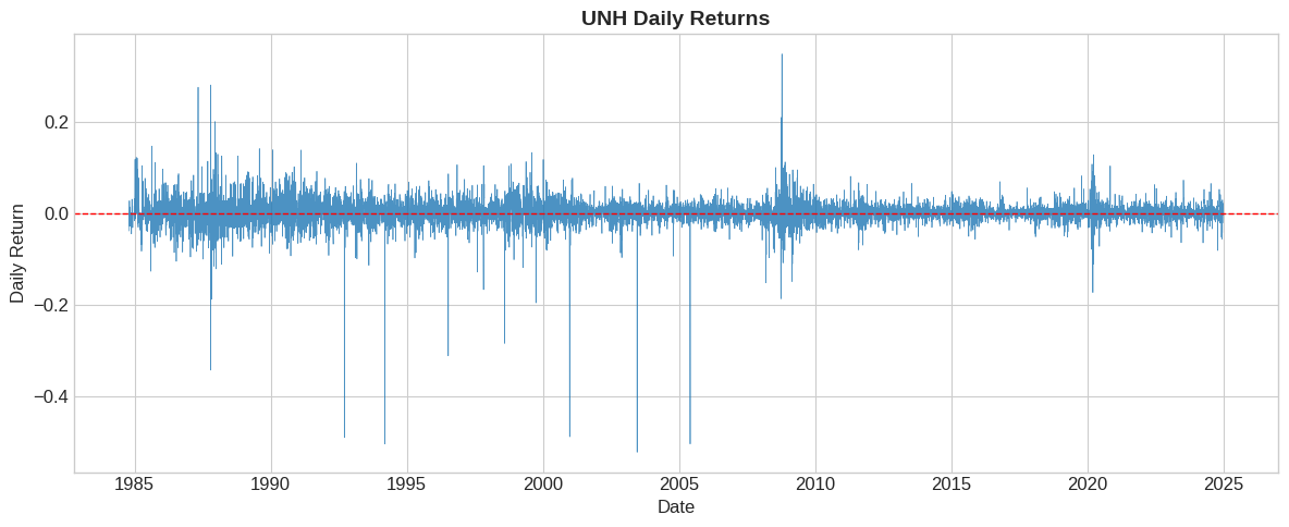
4.4.4. Visualizing the Return Series#
# Plot daily returns
fig, ax = plt.subplots(figsize=(12, 5))

ax.plot(df.index, df['ret'], linewidth=0.5, alpha=0.8)
ax.axhline(0, color='red', linestyle='--', linewidth=1)

ax.set_xlabel('Date')
ax.set_ylabel('Daily Return')
ax.set_title('UNH Daily Returns', fontsize=14, fontweight='bold')

plt.tight_layout()
plt.show()
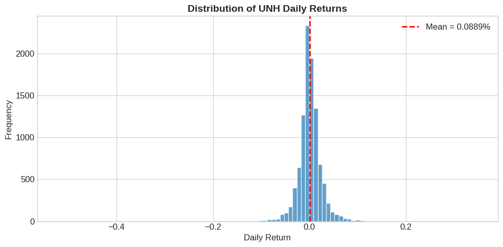
4.4.5. Return Distribution#
# Histogram of daily returns
fig, ax = plt.subplots(figsize=(10, 5))

ax.hist(df['ret'].dropna(), bins=100, edgecolor='white', alpha=0.7)
ax.axvline(df['ret'].mean(), color='red', linestyle='--',
           linewidth=2, label=f"Mean = {df['ret'].mean():.4%}")

ax.set_xlabel('Daily Return')
ax.set_ylabel('Frequency')
ax.set_title('Distribution of UNH Daily Returns', fontsize=14, fontweight='bold')
ax.legend()

plt.tight_layout()
plt.show()
4.4.6. Summary Statistics#
# Key summary statistics
mean_daily = df['ret'].mean()
std_daily = df['ret'].std()

# Annualize (252 trading days)
mean_annual = mean_daily * 252
std_annual = std_daily * np.sqrt(252)

print("━" * 40)
print("UNH Return Summary Statistics")
print("━" * 40)
print(f"Daily mean return:      {mean_daily:>10.4%}")
print(f"Daily std deviation:    {std_daily:>10.4%}")
print("━" * 40)
print(f"Annualized mean:        {mean_annual:>10.2%}")
print(f"Annualized volatility:  {std_annual:>10.2%}")
print("━" * 40)
━━━━━━━━━━━━━━━━━━━━━━━━━━━━━━━━━━━━━━━━
UNH Return Summary Statistics
━━━━━━━━━━━━━━━━━━━━━━━━━━━━━━━━━━━━━━━━
Daily mean return:         0.0889%
Daily std deviation:       2.7263%
━━━━━━━━━━━━━━━━━━━━━━━━━━━━━━━━━━━━━━━━
Annualized mean:            22.40%
Annualized volatility:      43.28%
━━━━━━━━━━━━━━━━━━━━━━━━━━━━━━━━━━━━━━━━
💡 Key Insight:
Means scale linearly with time: multiply by 252 (number of trading days in year)
Volatility scales with square root of time: multiply by \(\sqrt{252}\)
The mean scalling is exact for log-returns, but an approximation for geometric returns For the variance scaling to be exact we need log-returns and iid returns This is because variance (not std) is additive for independent returns. It is standard to use these scaling as quick approximations Suppose your data is monthly how would you annualize?
4.5. Excess Returns #
4.5.1. Why Excess Returns?#
A 10% return sounds great, but what if risk-free bonds paid 8%?
The stock only gave you 2% extra for taking on stock market risk.
Excess return = Return − Risk-free rate
4.5.2. Loading the Risk-Free Rate#
We use Kenneth French’s data library, which provides the 1-month T-bill rate.
import pandas_datareader.data as pdr

# Define a start date for data retrieval
start_date = '1900-01-01'
# Fetch daily Fama-French factors, including the risk-free rate
# The Fama-French data often comes as a dictionary of DataFrames, we need the first one for daily factors.
df_ff_daily = pdr.DataReader('F-F_Research_Data_Factors_Daily', 'famafrench', start=start_date)[0]
print("Fama-French daily factors loaded successfully!")
print(f"Data range: {df_ff_daily.index.min().date()} to {df_ff_daily.index.max().date()}")
df_ff_daily.head()
Fama-French daily factors loaded successfully!
Data range: 1926-07-01 to 2025-11-28
| Mkt-RF | SMB | HML | RF | |
|---|---|---|---|---|
| Date | ||||
| 1926-07-01 | 0.09 | -0.25 | -0.27 | 0.01 |
| 1926-07-02 | 0.45 | -0.33 | -0.06 | 0.01 |
| 1926-07-06 | 0.17 | 0.30 | -0.39 | 0.01 |
| 1926-07-07 | 0.09 | -0.58 | 0.02 | 0.01 |
| 1926-07-08 | 0.22 | -0.38 | 0.19 | 0.01 |
⚠️ Caution:
The risk-free rate is sometimes reported as an annual percentage. if that is the case need to divide by 100 and 252 (number of tradign days) how do you know what to do?
display(df_ff_daily.loc['2024',:].mean())

display(df_ff_daily.loc['2024',:].mean()*252)

display(df_ff_daily.loc['2024',:].mean()*252/100)
| 0 | |
|---|---|
| Mkt-RF | 0.071706 |
| SMB | -0.033373 |
| HML | -0.028532 |
| RF | 0.020000 |
| 0 | |
|---|---|
| Mkt-RF | 18.07 |
| SMB | -8.41 |
| HML | -7.19 |
| RF | 5.04 |
| 0 | |
|---|---|
| Mkt-RF | 0.1807 |
| SMB | -0.0841 |
| HML | -0.0719 |
| RF | 0.0504 |
# The RF column in df_ff_daily is in percentage (e.g., 0.01 means 0.01%), so convert to decimal by dividing by 100.
# Should you?
df_ff_daily['RF_decimal'] = df_ff_daily['RF'] / 100
# Convert annual risk-free rate to daily rate by dividing by 252 (trading days in a year)
df_ff_daily['rf_daily'] = df_ff_daily['RF_decimal']

# Merge risk-free rate with stock data (df - UNH data)
# Ensure both dataframes have the same index name for merging
df_ff_daily.index.name = 'date'
df_merged = df.merge(df_ff_daily[['rf_daily']], left_index=True, right_index=True, how='left')

print("Risk-free daily rates calculated and merged with UNH data.")
print("First few rows of df with new 'rf_daily' column:")
df_merged.head()
Risk-free daily rates calculated and merged with UNH data.
First few rows of df with new 'rf_daily' column:
| P | D | ret | rf_daily | |
|---|---|---|---|---|
| date | ||||
| 1984-10-18 | 4.8750 | 0.0 | NaN | 0.0004 |
| 1984-10-19 | 4.6875 | 0.0 | -0.038462 | 0.0004 |
| 1984-10-22 | 4.6875 | 0.0 | 0.000000 | 0.0004 |
| 1984-10-23 | 4.5625 | 0.0 | -0.026667 | 0.0004 |
| 1984-10-24 | 4.6875 | 0.0 | 0.027397 | 0.0004 |
4.5.3. Computing Excess Returns#
# Compute excess return
df_merged['ret_excess'] = df_merged['ret'] - df_merged['rf_daily']

# Compare return vs excess return
print("━" * 50)
print("Comparison: Return vs Excess Return")
print("━" * 50)
print(f"Mean return:         {df_merged['ret'].mean():>12.4%}")
print(f"Mean excess return:  {df_merged['ret_excess'].mean():>12.4%}")
print(f"Mean rf (daily):     {df_merged['rf_daily'].mean():>12.4%}")
print("━" * 50)
print(f"Std return:          {df_merged['ret'].std():>12.4%}")
print(f"Std excess return:   {df_merged['ret_excess'].std():>12.4%}")
print("━" * 50)
━━━━━━━━━━━━━━━━━━━━━━━━━━━━━━━━━━━━━━━━━━━━━━━━━━
Comparison: Return vs Excess Return
━━━━━━━━━━━━━━━━━━━━━━━━━━━━━━━━━━━━━━━━━━━━━━━━━━
Mean return:              0.0889%
Mean excess return:       0.0766%
Mean rf (daily):          0.0124%
━━━━━━━━━━━━━━━━━━━━━━━━━━━━━━━━━━━━━━━━━━━━━━━━━━
Std return:               2.7263%
Std excess return:        2.7262%
━━━━━━━━━━━━━━━━━━━━━━━━━━━━━━━━━━━━━━━━━━━━━━━━━━
💡 Key Insight:
Notice the standard deviations are nearly identical.
This is because the risk-free rate is (nearly) constant day-to-day. Subtracting a constant shifts the mean but doesn’t change volatility much.
But the risk-free rate..is risk-free..should it change the variance at all?
4.6. Excess returns as long-short trading strategies#
Excess returns are a nice way to look at an asset because it strips out the time-value of money aspect form it
Excess returns is really the return on a strategy that invests 1 in the risky asset and finance the position by borrowing at the risk-free rate
how much buying w dollars of Apple stock excess return cost you?
4.7. Long-short trading strategies are self-financed#
This means that you don’t need any cash to invest in it
you borrow all you need
of course you will bear risk. Banks will lend you if they expect to get paid
so in practice you will have limits on how many dollars on the strategy
For example you will be required to post collateral to support the trade
It is no different from when you buy a house with a mortage
4.8. Risk Premiums #
4.8.2. The Sharpe Ratio#
How much return do we get per unit of risk?
# Compute Sharpe ratio
sharpe_daily = df_merged['ret_excess'].mean() / df_merged['ret_excess'].std()
sharpe_annual = sharpe_daily * np.sqrt(252)  # Sharpe scales with sqrt(T)

print(f"UNH Sharpe Ratio")
print(f"━" * 30)
print(f"Daily:     {sharpe_daily:>8.4f}")
print(f"Annual:    {sharpe_annual:>8.2f}")
UNH Sharpe Ratio
━━━━━━━━━━━━━━━━━━━━━━━━━━━━━━
Daily:       0.0281
Annual:        0.45
📌 Remember:
Sharpe Ratio > 0.5 (annual) is considered good
Sharpe Ratio > 1.0 (annual) is exceptional
The S&P 500 has a historical Sharpe Ratio of about 0.4-0.5
Why we might care about the Sharpe Ratio?
4.8.3. Cumulative Returns: The Power of Compounding#
# Compute cumulative returns (wealth growth from $1)
df_merged['cum_ret'] = (1 + df_merged['ret']).cumprod()
df_merged['cum_rf'] = (1 + df_merged['rf_daily']).cumprod()

# Plot cumulative returns
fig, ax = plt.subplots(figsize=(12, 6))

ax.plot(df_merged.index, df_merged['cum_ret'], label='UNH', linewidth=2)
ax.plot(df_merged.index, df_merged['cum_rf'], label='Risk-Free', linewidth=2, linestyle='--')

ax.set_xlabel('Date')
ax.set_ylabel('Cumulative Return ($1 initial investment)')
ax.set_title('Wealth Growth: UNH vs Risk-Free', fontsize=14, fontweight='bold')
ax.legend(loc='upper left')
ax.set_yscale('log')

plt.tight_layout()
plt.show()
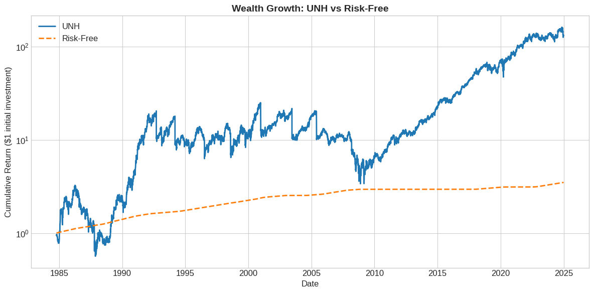
💡 Key Insight:
The gap between the lines is the cumulative excess return. This is the total compensation you received for bearing stock risk.
4.9. 📝 Exercises #
4.9.1. Exercise 1: Warm-up — Basic Return Calculation#
🔧 Exercise:
A stock has the following prices over 4 days (no dividends):
Day 0: $50
Day 1: $52
Day 2: $48
Day 3: $51
Compute the daily returns for Days 1, 2, and 3
Compute the cumulative return over the 3-day period
Verify: \((1+R_1) \times (1+R_2) \times (1+R_3) - 1\) equals the cumulative return
# Your code here
prices = [50, 52, 48, 51]

# Compute daily returns


# Compute cumulative return


# Verify
💡 Click to see solution
prices = [50, 52, 48, 51]

# Compute daily returns
R1 = (52 - 50) / 50  # 4%
R2 = (48 - 52) / 52  # -7.69%
R3 = (51 - 48) / 48  # 6.25%

print(f"Day 1 return: {R1:.4%}")
print(f"Day 2 return: {R2:.4%}")
print(f"Day 3 return: {R3:.4%}")

# Cumulative return: (51 - 50) / 50 = 2%
cum_ret = (51 - 50) / 50
print(f"\nCumulative return: {cum_ret:.4%}")

# Verify via compounding
compounded = (1 + R1) * (1 + R2) * (1 + R3) - 1
print(f"Compounded returns: {compounded:.4%}")
4.9.2. Exercise 2: Extension — Another Stock#
🤔 Think and Code:
Load data for another stock and compare to UNH:
Load the SPY-WMT-JPM dataset from the URL below
Compute daily returns for SPY (the S&P 500 ETF)
Compare the annualized mean and volatility to UNH
Which investment had a higher Sharpe Ratio?
# Your code here
url2 = 'https://raw.githubusercontent.com/amoreira2/UG54/main/assets/data/df_SPYWMTJPM_data.csv'
💡 Click to see solution
url2 = 'https://raw.githubusercontent.com/amoreira2/UG54/main/assets/data/df_SPYWMTJPM_data.csv'
df2 = pd.read_csv(url2, parse_dates=['date'], index_col='date')


# Annualized statistics
spy_mean = df2['SPY'].mean() * 252
spy_std = df2['SPY'].std() * np.sqrt(252)
spy_sharpe = spy_mean / spy_std

print(f"SPY: Mean = {spy_mean:.2%}, Vol = {spy_std:.2%}, Sharpe = {spy_sharpe:.2f}")
print(f"UNH: Mean = {mean_annual:.2%}, Vol = {std_annual:.2%}")
4.9.3. Exercise 3: Open-ended — Risk Analysis#
🤔 Think and Code:
You have $1 million invested in UNH:
Estimate the 5th percentile of daily returns (Value at Risk proxy)
What dollar amount could you lose on a “bad day” (5% probability)?
Find the worst single-day loss in the sample
Plot the distribution with the 5th percentile and worst day marked
Discuss: Is the normal distribution a good model for stock returns?
# Your code here
portfolio_value = 1_000_000

# 5th percentile


# Dollar loss


# Worst day


# Plot
💡 Click to see solution
portfolio_value = 1_000_000

# 5th percentile (empirical VaR)
var_5 = df_merged['ret'].quantile(0.05)
print(f"5th percentile return: {var_5:.4%}")

# Dollar loss
dollar_loss = portfolio_value * abs(var_5)
print(f"5% daily VaR: ${dollar_loss:,.0f}")

# Worst day
worst_day = df_merged['ret'].min()
worst_date = df_merged['ret'].idxmin()
print(f"Worst day: {worst_day:.4%} on {worst_date.date()}")

# Plot
fig, ax = plt.subplots(figsize=(10, 5))
ax.hist(df['ret'].dropna(), bins=100, edgecolor='white', alpha=0.7)
ax.axvline(var_5, color='orange', linestyle='--', linewidth=2, label=f'5% VaR: {var_5:.2%}')
ax.axvline(worst_day, color='red', linestyle='--', linewidth=2, label=f'Worst: {worst_day:.2%}')
ax.legend()
ax.set_title('UNH Return Distribution with Risk Measures')
plt.show()

# Discussion: Returns have "fat tails" - extreme events are more
# common than a normal distribution would predict.
4.9.4. Exercise 4: Challenge — Rolling Analysis#
🔧 Exercise:
Compute and plot the rolling 252-day Sharpe Ratio for UNH:
Create a rolling 252-day window
For each window, compute: mean excess return / std excess return × √252
Plot the rolling Sharpe Ratio over time
Identify periods of exceptionally high or low risk-adjusted performance
What do we learn from this plot?
# Your code here
💡 Click to see solution
# Rolling Sharpe Ratio
window = 252
rolling_mean = df_merged['ret_excess'].rolling(window).mean()
rolling_std = df_merged['ret_excess'].rolling(window).std()
df_merged['rolling_sharpe'] = (rolling_mean / rolling_std) * np.sqrt(252)

# Plot
fig, ax = plt.subplots(figsize=(12, 5))
ax.plot(df_merged.index, df_merged['rolling_sharpe'], linewidth=1.5)
ax.axhline(0, color='red', linestyle='--', linewidth=1)
ax.axhline(0.5, color='green', linestyle=':', linewidth=1, alpha=0.5, label='Good (0.5)')
ax.axhline(1.0, color='green', linestyle=':', linewidth=1, alpha=0.8, label='Excellent (1.0)')

ax.set_xlabel('Date')
ax.set_ylabel('Rolling 1-Year Sharpe Ratio')
ax.set_title('UNH Rolling Sharpe Ratio', fontsize=14, fontweight='bold')
ax.legend()

plt.tight_layout()
plt.show()
4.10. 🧠 Key Takeaways #
Total Return = \((P_t + D_t - P_{t-1}) / P_{t-1}\) — Captures price change AND dividends
Excess Return = Return − Risk-free rate — Measures compensation for risk
Risk Premium = E[Excess Return] — The expected reward for bearing risk
Sharpe Ratio = Risk Premium / Volatility — Risk-adjusted performance measure
Annualizing: Means multiply by 252, volatility by √252, Sharpe by √252
Think carefully: how exactly to measure what I want in the data