
7. Portfolios#
7.1. 🎯 Learning Objectives#
By the end of this notebook, you will be able to:
See risk through a portfolio lens — Grasp Markowitz’s insight that an asset’s danger depends on what it adds to the whole mix, not on its stand-alone volatility
Express returns, means, and variance with matrix algebra — Use \(R_p = W'R\), \(E[R_p]=W'E[R]\), and \(\text{Var}(R_p)=W'\Sigma W\) to scale from two assets to hundreds
Quantify diversification benefits — Investigate how adding a higher-volatility asset can lower portfolio variance when correlations are below one
Compute and interpret portfolio weights — Distinguish long-only, short, and leveraged positions; verify that weights sum to one
7.2. 📋 Table of Contents#
#@title 🛠️ Setup: Run this cell first <a id="setup"></a>

import numpy as np
import pandas as pd
import matplotlib.pyplot as plt
%matplotlib inline

# Set consistent plot style
plt.style.use('seaborn-v0_8-whitegrid')
plt.rcParams['figure.figsize'] = [10, 6]
7.3. Why Think in Portfolios? #
Harry Markowitz’s great insight was to think of risk in terms of what an asset adds to your portfolio, not its stand-alone volatility.
💡 Key Insight:
Just like sugar can be good for you if you’re not eating any, but terrible if you’re eating a lot of it—what investors should care about is their final diet.
If a stock brings a lot of what you already have, it will be risky for you.
Why volatility alone is misleading:
If you have only 1% in a stock and it drops to ZERO, you lose only 1% of your portfolio
The stock’s volatility doesn’t matter much at small positions
As you buy more, it becomes risky for you because your portfolio moves more like it
If this stock moves together with your other holdings, even a small position can feel very risky
📌 Remember:
The covariance across stocks is a key determinant of how much we can hold volatile stocks without adding much overall risk.
7.4. Portfolio Weights #
The portfolio weight for stock \(j\), denoted \(w_j\), is the fraction of portfolio value held in stock \(j\):
📌 Remember:
Portfolio weights sum to one:
\[\sum_{j=1}^N w_j = 1 \quad \text{or in matrix notation:} \quad \mathbf{1}'W = 1\]This doesn’t mean you can’t borrow—just that negative weights offset positive ones.
📌 Warning:
We often separate the weight on the risk-free asset
\[\sum_{j=1}^N w_j +w_{rf}= 1 \quad \text{risky weights can be larger than 1 if $w_{rf}$ negative} \quad \sum_{j=1}^N w_j =1-w_{rf}\]
Type |
Description |
Example |
|---|---|---|
Long-only |
All weights \(\geq 0\) |
\(W=[0.6,\,0.3],\; w_{rf}=0.1\) |
Short |
Some \(w_i < 0\) |
\(W=[1.2,\,-0.4],\; w_{rf}=0.2\) |
Leveraged |
Risky weights sum to \(>1\) |
\(W=[1.5,\,0.5],\; w_{rf}=-1\) |
We will often work with excess returns. These are portfolios that are long a risky asset and short the risk-free asset
7.5. Our Dataset #
We’ll work with monthly excess returns for:
🇺🇸 US equities (S&P 500, MKT)
🌍 International developed markets (WorldxUSA)
🌏 Emerging markets
📈 US government bonds
🌐 International government bonds
#@title 📊 Load Data

url = "https://raw.githubusercontent.com/amoreira2/UG54/main/assets/data/GlobalFinMonthly.csv"
Data = pd.read_csv(url)
Data['Date'] = pd.to_datetime(Data['Date'])
Data = Data.set_index('Date')

# Replace sentinel values (e.g. -99) with NaN before any computation
Data = Data[Data > -1].dropna()

print(f"Data shape: {Data.shape}")
print(f"Date range: {Data.index[0].strftime('%Y-%m')} to {Data.index[-1].strftime('%Y-%m')}")
Data.head()
# Convert to excess returns
Rf = Data['RF']
Data = Data.drop(columns=['RF']).subtract(Rf, axis=0)
Data = Data.dropna()
Data.head()
7.6. Portfolio Returns #
Portfolio returns are the dollar-weighted average of individual position returns:
Where:
\(R\) is the \(N \times 1\) vector of asset returns
\(W\) is the \(N \times 1\) vector of weights
We can rewrite the portfolio of regular assets in terms of a portfolio of excess returns,
where \(R^e\) is the vector of risky assets excess returns and \(W=[w_2,w_3,...w_N]\) is the vector of risky assets weights
Note that even though we impose that the weights \(w_i\) add up to 1, the weights W can add up to values below 1 or above 1
Why? because we represented everything in terms of self-funded portfolios
Here we are working directly with excess returns
# Construct an equal-weighted portfolio
N = len(Data.columns)
W = np.ones((N, 1)) / N

print(f"Number of assets: {N}")
print(f"Weights: {W.flatten()}")
print(f"Weights sum to: {W.sum():.4f}")
Number of assets: 5
Weights: [0.2 0.2 0.2 0.2 0.2]
Weights sum to: 1.0000
🐍 Python Insight: Matrix multiplication with
@The
@operator performs matrix multiplication in Python:portfolio_return = Data @ W # T×N matrix @ N×1 vector = T×1 vectorThis replaces messy for loops with a single line!
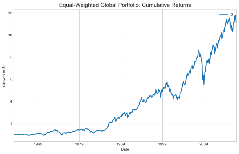
# Compute portfolio returns for ALL dates at once
Rp = Data @ W
# Plot cumulative returns
fig, ax = plt.subplots(figsize=(10, 6))
(1 + Rp).cumprod().plot(ax=ax, linewidth=2)
ax.set_title('Equal-Weighted Global Portfolio: Cumulative Returns', fontsize=14)
ax.set_ylabel('Growth of $1')
plt.show()
7.7. Portfolio Expected Returns #
Since expectations are linear, the expected portfolio return is:
If the porfolio expected excess return is \(E[r_p^e]\) say 5%, what is the expected return?
# Estimate expected returns from historical data
E_hat = Data.mean()

print("Monthly expected excess returns:")
print(E_hat.round(4))
print("\nAnnualized expected excess returns:")
print((E_hat * 12).round(4))
Monthly expected excess returns:
MKT                 0.0052
USA30yearGovBond    0.0025
EmergingMarkets     0.0068
WorldxUSA           0.0042
WorldxUSAGovBond    0.0021
dtype: float64

Annualized expected excess returns:
MKT                 0.0622
USA30yearGovBond    0.0304
EmergingMarkets     0.0814
WorldxUSA           0.0500
WorldxUSAGovBond    0.0246
dtype: float64
# Two equivalent ways to compute portfolio expected return
E_rp_method1 = W.T @ E_hat  # Matrix multiplication
E_rp_method2 = Rp.mean()     # Direct average of portfolio returns

print(f"Via W'E[R]: {E_rp_method1[0]:.6f}")
print(f"Via mean(Rp): {E_rp_method2[0]:.6f}")
print(f"\nAnnualized: {E_rp_method1[0] * 12:.2%}")
Via W'E[R]: 0.004144
Via mean(Rp): 0.004144

Annualized: 4.97%
7.8. Portfolio Variance #
Portfolio variance is NOT the weighted average of individual variances!
Two-asset case:
N-asset case:
where \(\Sigma\) is the \(N \times N\) variance-covariance matrix.
💡 Key Insight:
For 50 assets, the formula has 50 variance terms and 2,450 covariance terms! Matrix algebra saves us from nested for loops.
# Estimate the covariance matrix
Cov_hat = Data.cov().to_numpy()

print("Covariance matrix (monthly):")
display(Cov_hat.round(6))
Covariance matrix (monthly):
array([[ 1.950e-03,  1.110e-04,  1.298e-03,  1.265e-03,  1.870e-04],
       [ 1.110e-04,  1.229e-03, -2.040e-04, -1.300e-05,  2.640e-04],
       [ 1.298e-03, -2.040e-04,  3.550e-03,  1.664e-03,  2.490e-04],
       [ 1.265e-03, -1.300e-05,  1.664e-03,  2.185e-03,  4.220e-04],
       [ 1.870e-04,  2.640e-04,  2.490e-04,  4.220e-04,  4.070e-04]])
# Compute portfolio variance using matrix algebra
Var_rp = (Data@W).var()[0]
Vol_rp = np.sqrt(Var_rp)
# Compute portfolio variance using matrix algebra
Var_rp_m = (W.T @ Cov_hat @ W)
Vol_rp_m = np.sqrt(Var_rp_m)

print(f"Monthly variance: {Var_rp}")
print(f"Annualized volatility: {Vol_rp * np.sqrt(12)}")


print(f"Monthly variance: {Var_rp_m}")
print(f"Annualized volatility: {Vol_rp_m * np.sqrt(12)}")
Monthly variance: 0.0007923455067886972
Annualized volatility: 0.09750972300988432
Monthly variance: [[0.00079235]]
Annualized volatility: [[0.09750972]]
7.9. Diversification #
The famous advice: “Don’t put all your eggs in one basket.”
Let’s examine this from a US investor’s perspective considering international stocks.
# Correlation and volatility of US vs International
print("Correlation matrix:")
display(Data[['MKT', 'WorldxUSA']].corr().round(3))

print("\nAnnualized volatilities:")
print((Data[['MKT', 'WorldxUSA']].std() * np.sqrt(12)).round(4))
🤔 Think and Code:
The international market is more volatile than the US market. Which portfolio do you expect to have the lowest volatility?
100% US?
100% International?
Something in between?
# Trace how volatility varies with international allocation
D = Data[['MKT', 'WorldxUSA']]
Cov_2 = D.cov()

results = []
for w_intl in np.arange(0, 1.01, 0.01):
    W_2 = np.array([[1 - w_intl], [w_intl]])
    var = (W_2.T @ Cov_2 @ W_2)[0, 0]
    vol_annual = np.sqrt(var) * np.sqrt(12)
    results.append([w_intl, vol_annual])

results = pd.DataFrame(results, columns=['Weight_Intl', 'Volatility'])
# Plot the diversification benefit
fig, ax = plt.subplots(figsize=(10, 6))
ax.plot(results['Weight_Intl'], results['Volatility'], linewidth=2, color='steelblue')
ax.axhline(y=results['Volatility'].min(), color='red', linestyle='--', alpha=0.7,
           label=f"Minimum vol: {results['Volatility'].min():.2%}")

# Mark pure portfolios
ax.scatter([0, 1], [results.iloc[0]['Volatility'], results.iloc[-1]['Volatility']],
           s=100, zorder=5, color='darkred')
ax.annotate('100% US', (0, results.iloc[0]['Volatility']),
            xytext=(0.05, results.iloc[0]['Volatility'] + 0.005))
ax.annotate('100% Intl', (1, results.iloc[-1]['Volatility']),
            xytext=(0.85, results.iloc[-1]['Volatility'] + 0.005))

ax.set_xlabel('Weight on International', fontsize=12)
ax.set_ylabel('Annualized Volatility', fontsize=12)
ax.set_title('Diversification Benefit: US + International', fontsize=14)
ax.legend()
plt.show()
💡 Key Insight:
Adding a more volatile asset can reduce portfolio volatility when correlations are below 1! This is the power of diversification.
7.10. The Mean-Variance Frontier #
Now let’s trace the investment frontier: how expected returns change with risk.
# Compute mean-variance frontier
E_2 = D.mean() * 12  # Annualized expected returns

frontier = []
for w_intl in np.arange(0, 1.01, 0.01):
    W_2 = np.array([[1 - w_intl], [w_intl]])

    # Expected return
    er = (W_2.T @ E_2)[0]

    # Volatility
    var = (W_2.T @ Cov_2 @ W_2)[0, 0]
    vol = np.sqrt(var) * np.sqrt(12)

    frontier.append([w_intl, vol, er])

frontier = pd.DataFrame(frontier, columns=['Weight_Intl', 'Volatility', 'Expected_Return'])
# Plot the mean-variance frontier
fig, ax = plt.subplots(figsize=(10, 6))

# Color by weight on international
scatter = ax.scatter(frontier['Volatility'], frontier['Expected_Return'],
                     c=frontier['Weight_Intl'], cmap='coolwarm', s=50)
plt.colorbar(scatter, label='Weight on International')

# Mark pure portfolios
ax.scatter([frontier.iloc[0]['Volatility']], [frontier.iloc[0]['Expected_Return']],
           s=150, color='blue', marker='s', zorder=5, label='100% US')
ax.scatter([frontier.iloc[-1]['Volatility']], [frontier.iloc[-1]['Expected_Return']],
           s=150, color='red', marker='s', zorder=5, label='100% Intl')

ax.set_xlabel('Annualized Volatility', fontsize=12)
ax.set_ylabel('Annualized Expected Excess Return', fontsize=12)
ax.set_title('Mean-Variance Frontier: US + International', fontsize=14)
ax.legend()
plt.show()
7.11. 📝 Exercises #
7.11.1. Exercise 1: Warm-up — Custom Portfolio#
🔧 Exercise:
Create a portfolio with:
50% in MKT (US equities)
30% in WorldxUSA (International)
20% in Bonds (if available, else EmergingMarkets)
Compute:
The portfolio’s annualized expected excess return
The portfolio’s annualized volatility
The portfolio’s Sharpe ratio
# Your code here
7.11.2. Exercise 2: Extension — Minimum Variance Portfolio#
🤔 Think and Code:
Using only MKT and WorldxUSA:
Find the weight on international that minimizes portfolio volatility
What is the minimum achievable volatility?
Compare this to holding 100% US—what’s the volatility reduction?
# Your code here
7.11.3. Exercise 3: Open-ended — Three-Asset Frontier#
🤔 Think and Code:
Extend the analysis to three assets: MKT, WorldxUSA, and EmergingMarkets.
Create a grid of weights (w_us, w_intl, w_em) that sum to 1
Compute expected return and volatility for each combination
Plot the three-asset frontier
Does adding emerging markets improve the frontier?
# Your code here
7.12. 🧠 Key Takeaways #
Matrix algebra is your friend — A single line replaces nested loops when calculating returns, expectations, and variance
Diversification is all about correlations — Pairing volatile but imperfectly correlated assets can cut overall risk more than simply holding the lower-volatility asset alone
How risky is an asset? — It fundamentally depends on the portfolio of who is asking
The key formulas:
Quantity |
Formula |
|---|---|
Portfolio return |
\(R_p = W'R\) |
Expected return |
\(E[R_p] = W'E[R]\) |
Variance |
\(\text{Var}(R_p) = W'\Sigma W\) |