
5. Timing#
5.1. Static Single Asset Example#
We model preferences using mean-variance utility
Consider a mean-variance investor allocating between a factor (the market) and a risk-free asset.
The investor solves:
where:
\(w\) = weight on the risky portfolio
\(r_{t+1}\) = risky asset return
Not known at date t. it is a random variable: \(E[r_{t+1}]\neq r_{t+1}\)
\(r^f\) = risk-free rate from t to t+1
known at date t: \(E[r^f]= r^f\)
\(\gamma\) = risk aversion coefficient
\(\text{E}(x)\) = Expectation of random variable x
\(\text{Var}(x)\) = variance of random variable x
The solution is elegantly simple:
💡 Key Insight: At the optimal, the slope of your objective cannot change with the weight
💡 Key Insight: The optimal allocation formula
\[w^* = \frac{E[r_{t+1} - r^f]}{\gamma \cdot Var(r_{t+1})}\]You invest proportionally to the risk-return trade-off:
📈 Lever up when expected returns are higher
📉 Lever down when variance is higher
5.3. Single asset with time-varying moments#
Same problem but now expected returns, risk-free, and variance move around over time
where:
\(w_t\) = weight on the risky portfolio at date t
\(r_{t+1}\) = risky asset return from t to t+1
Not known at date t. it is a random variable: \(E_t[r_{t+1}]\neq r_{t+1}\)
\(r^f_{t+1}\) = risk-free rate from t to t+1 (known at date t. )
known at date t: \(E[r^f_{t+1}]= r^f_{t+1}\)
\(E_t(x)\) = Expectation of random variable x at date t given all I know
\(Var_t(x)\) = E_t[(x-E_t[x])^2] variance of random variable x around what I expect the vriable to be given all I know
This can be simplified to:
Do you understand why this follows?
We get the same result!
The volatility of you portfolio should track the Sharpe ratio of the portfolio over time
What is the intuition?
Note that given the behavior of excess returns, variation in the risk-free rate does not matter at all
5.4. ⚠️ Caution: The risk-free rate#
Is \(Var(r_{t+1})=Var(r^e_{t+1})\)?
If I compute both in the data, will they be the same?
Should it matter if the risk-free is constant or time-varying?
If it moves around does it mean it is risky?
What is the correct one to use?
import pandas as pd
import pandas_datareader as pdr
import matplotlib.pyplot as plt

# Import 3-month Treasury Bill rate from FRED (entire time series)
tbill_3m = pdr.data.DataReader('TB3MS', 'fred', start='1934-01-01')

# Plot the 3-month T-Bill rate over time
plt.figure(figsize=(12, 6))
plt.plot(tbill_3m.index, tbill_3m['TB3MS'])
plt.title('3-Month Treasury Bill Rate Over Time')
plt.xlabel('Date')
plt.ylabel('Rate (%)')
plt.grid(True, alpha=0.3)
plt.tight_layout()
plt.show()

print(f'The variance of the 3-month Treasury Bill rate is: {tbill_3m['TB3MS'].var()}')
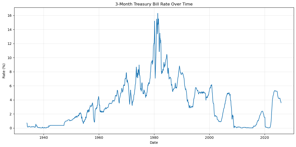
The variance of the 3-month Treasury Bill rate is: 9.583294505022533
5.5. 📌 Key Takeaways#
Before diving into implementation, remember these core principles:
Time-varying moments create opportunity: If expected returns and volatility change over time, you can exploit this through dynamic allocation
The optimal allocation is intuitive: Invest proportionally to expected excess return, inversely to variance and risk aversion
Target the Sharpe ratio: Adjust portfolio volatility based on how attractive the risk-return trade-off is
Think carefully about what you do: What you do in the data needs to be guided by an economic understanding
In the following notebooks, we’ll explore two practical approaches:
Expected Returns Timing: Predicting when market returns will be high or low
Volatility Timing: Adjusting exposure based on time-varying risk