
5.7. Volatility Timing#
5.7.1. 🎯 Learning Objectives#
By the end of this notebook, you will be able to:
Understand the volatility timing logic — Why scaling by inverse variance improves risk-adjusted returns
Construct realized variance from daily data — Aggregate daily returns to monthly variance estimates
Build volatility-managed portfolios — Create weights inversely proportional to recent volatility
Evaluate the strategy empirically — Test if the price of risk declines with volatility
Apply volatility timing to multiple factors — Extend the approach beyond just the market
5.7.2. 📋 Table of Contents#
5.7.3. 🛠️ Setup #
#@title 🛠️ Setup: Run this cell first (click to expand)

# Core libraries
import numpy as np
import pandas as pd
import matplotlib.pyplot as plt
%matplotlib inline

# pandas-datareader: Fetches financial data from online sources
from pandas_datareader import data as DataReader

# Set consistent plot style
plt.style.use('seaborn-v0_8-whitegrid')
plt.rcParams['figure.figsize'] = [10, 6]
plt.rcParams['font.size'] = 12

# Suppress warnings for cleaner output
import warnings
warnings.filterwarnings('ignore')

print("✅ Libraries loaded successfully!")
✅ Libraries loaded successfully!
#@title Helper Function: Get Factor Data

def get_factors(factors='CAPM', freq='daily'):
    """
    Fetch Fama-French factor data from Ken French's website.

    Parameters:
    -----------
    factors : str
        'CAPM', 'FF3', 'FF5', or 'FF6'
    freq : str
        'daily' or 'monthly'
    """
    freq_label = '' if freq == 'monthly' else '_' + freq

    if factors == 'CAPM':
        ff = DataReader.DataReader(f"F-F_Research_Data_Factors{freq_label}",
                                   "famafrench", start="1921-01-01")
        df_factor = ff[0][['RF', 'Mkt-RF']]
    elif factors == 'FF3':
        ff = DataReader.DataReader(f"F-F_Research_Data_Factors{freq_label}",
                                   "famafrench", start="1921-01-01")
        df_factor = ff[0][['RF', 'Mkt-RF', 'SMB', 'HML']]
    elif factors == 'FF5':
        ff = DataReader.DataReader(f"F-F_Research_Data_Factors{freq_label}",
                                   "famafrench", start="1921-01-01")
        df_factor = ff[0][['RF', 'Mkt-RF', 'SMB', 'HML']]
        ff2 = DataReader.DataReader(f"F-F_Research_Data_5_Factors_2x3{freq_label}",
                                    "famafrench", start="1921-01-01")
        df_factor = df_factor.merge(ff2[0][['RMW', 'CMA']], on='Date', how='outer')
    else:  # FF6
        ff = DataReader.DataReader(f"F-F_Research_Data_Factors{freq_label}",
                                   "famafrench", start="1921-01-01")
        df_factor = ff[0][['RF', 'Mkt-RF', 'SMB', 'HML']]
        ff2 = DataReader.DataReader(f"F-F_Research_Data_5_Factors_2x3{freq_label}",
                                    "famafrench", start="1921-01-01")
        df_factor = df_factor.merge(ff2[0][['RMW', 'CMA']], on='Date', how='outer')
        mom = DataReader.DataReader(f"F-F_Momentum_Factor{freq_label}",
                                    "famafrench", start="1921-01-01")
        df_factor = df_factor.merge(mom[0], on='Date')
        df_factor.columns = ['RF', 'Mkt-RF', 'SMB', 'HML', 'RMW', 'CMA', 'MOM']

    if freq == 'monthly':
        df_factor.index = pd.to_datetime(df_factor.index.to_timestamp())
    else:
        df_factor.index = pd.to_datetime(df_factor.index)

    return df_factor / 100
5.7.4. The Volatility Timing Logic #
5.7.4.1. The Optimal Allocation Formula#
Recall the mean-variance optimal weight:
Two extreme cases:
Case |
Formula |
Strategy |
|---|---|---|
Constant variance |
$\(x_t = \frac{E_t[r^e]}{\gamma \sigma^2}\)$ |
Time expected returns |
Constant expected returns |
$\(x_t = \frac{\mu}{\gamma \cdot \text{Var}_t}\)$ |
Time variance |
5.7.4.2. When Does Volatility Timing Work?#
Suppose expected returns relate to variance as:
Then the optimal weight becomes:
💡 Key Insight:
If \(a = 0\) (expected returns proportional to variance): No benefit from vol timing
If \(b = 0\) (expected returns constant): Maximum benefit from vol timing
Reality is somewhere in between, but closer to \(b = 0\) for most factors
📌 Remember:
This only works if the factor has positive alpha/premium to begin with. If the Sharpe ratio is zero, you can’t increase it by managing risk!
5.7.5. Constructing Realized Variance #
5.7.5.1. Loading Daily Factor Data#
# Get daily factor data
df_factor = get_factors('CAPM', freq='daily')

print(f"Data range: {df_factor.index.min().date()} to {df_factor.index.max().date()}")
df_factor.head()
Data range: 1926-07-01 to 2025-12-31
| RF | Mkt-RF | |
|---|---|---|
| Date | ||
| 1926-07-01 | 0.0001 | 0.0009 |
| 1926-07-02 | 0.0001 | 0.0045 |
| 1926-07-06 | 0.0001 | 0.0017 |
| 1926-07-07 | 0.0001 | 0.0009 |
| 1926-07-08 | 0.0001 | 0.0022 |
5.7.5.2. Computing Monthly Realized Variance#
We estimate variance using daily returns within each month:
This gives us a forward-looking volatility estimate based on recent data.
🐍 Python Insight:
groupby()The pandas
groupby()method is one of the most powerful tools for data analysis. It follows the Split → Apply → Combine pattern:df.groupby(grouping_key).aggregate_function()
Step
Action
Example
Split
Divide data into groups
df.groupby(df.index.year)Apply
Apply function to each group
.mean(),.sum(),.prod()Combine
Merge results back together
Returns one row per group
We’ll use this extensively throughout the course!
# Compute monthly realized variance (annualized)
RV = df_factor[['Mkt-RF']].groupby(
df_factor.index + pd.offsets.MonthEnd(0)
).var() * 252
RV = RV.rename(columns={'Mkt-RF': 'RV'})
# Aggregate daily returns to monthly
Ret = (1 + df_factor).groupby(
df_factor.index + pd.offsets.MonthEnd(0)
).prod() - 1
# Merge variance and returns
df = RV.merge(Ret, how='left', left_index=True, right_index=True)
# Lag variance by one month (we use last month's variance to form today's weights)
df['RV_lag'] = df['RV'].shift(1)
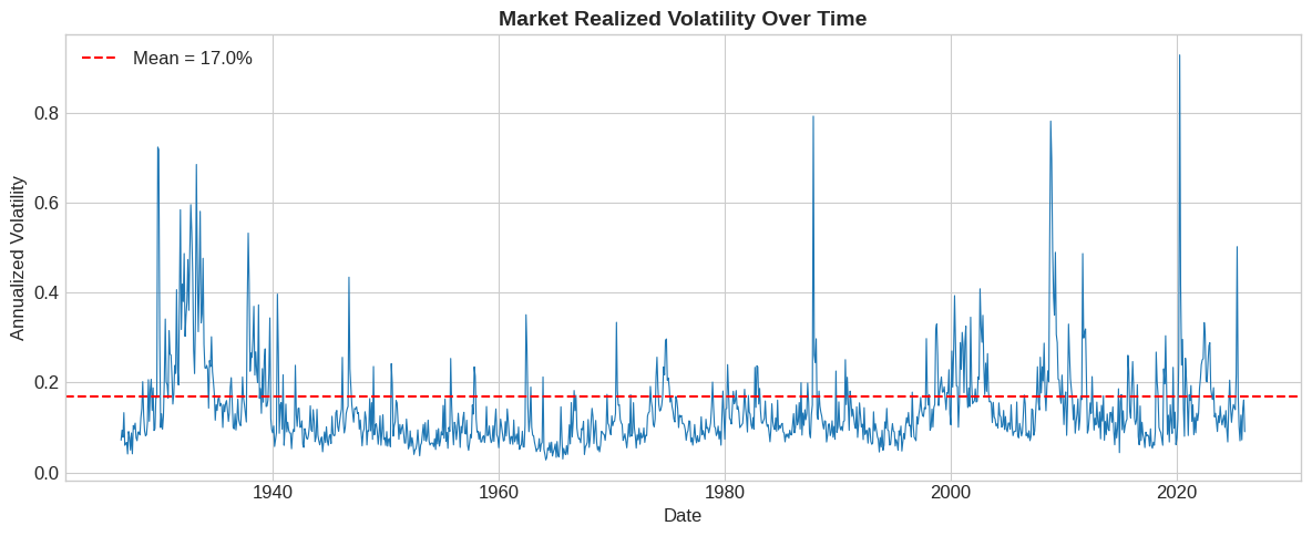
print(f"Average annualized variance: {df['RV'].mean():.4f}")
print(f"Average annualized volatility: {np.sqrt(df['RV'].mean()):.2%}")
Average annualized variance: 0.0287
Average annualized volatility: 16.95%
# Visualize realized volatility over time
fig, ax = plt.subplots(figsize=(12, 5))

ax.plot(df.index, np.sqrt(df['RV']), linewidth=0.8)
ax.axhline(np.sqrt(df['RV'].mean()), color='red', linestyle='--',
           label=f'Mean = {np.sqrt(df["RV"].mean()):.1%}')

ax.set_xlabel('Date')
ax.set_ylabel('Annualized Volatility')
ax.set_title('Market Realized Volatility Over Time', fontsize=14, fontweight='bold')
ax.legend()

plt.tight_layout()
plt.show()
5.7.6. Does Volatility Predict the Price of Risk? #
5.7.6.1. The Key Test#
For volatility timing to work, we need:
Translation: When volatility is high, the risk-return tradeoff worsens.
If a=0 this will not happen
# Sort months into quintiles by lagged volatility
df['Quantile'] = pd.qcut(df['RV_lag'], q=5, labels=['Q1 (Low)', 'Q2', 'Q3', 'Q4', 'Q5 (High)'])

# Compute means by quintile
quantile_stats = df.groupby('Quantile').agg({
        'RV_lag': 'mean',
    'RV': 'mean',
    'Mkt-RF': 'mean'

})

# Compute price of risk (return per unit variance)
quantile_stats['Price_of_Risk'] = quantile_stats['Mkt-RF'] * 12 / quantile_stats['RV']
quantile_stats['RV**0.5'] = np.sqrt(quantile_stats['RV_lag'])
quantile_stats['RV(t+1)**05'] = np.sqrt(quantile_stats['RV'])
quantile_stats['Return(t+1)'] = quantile_stats['Mkt-RF'] * 12
quantile_stats['SharpeRatio'] = quantile_stats['Mkt-RF'] * 12 / quantile_stats['RV(t+1)**05']
quantile_stats
| RV_lag | RV | Mkt-RF | Price_of_Risk | RV**0.5 | RV(t+1)**05 | Return(t+1) | SharpeRatio | |
|---|---|---|---|---|---|---|---|---|
| Quantile | ||||||||
| Q1 (Low) | 0.004163 | 0.008515 | 0.006555 | 9.237906 | 0.064518 | 0.092278 | 0.078663 | 0.852456 |
| Q2 | 0.008063 | 0.012690 | 0.007419 | 7.015934 | 0.089792 | 0.112651 | 0.089034 | 0.790352 |
| Q3 | 0.012829 | 0.015471 | 0.004881 | 3.786062 | 0.113264 | 0.124383 | 0.058575 | 0.470923 |
| Q4 | 0.022829 | 0.029652 | 0.007121 | 2.882005 | 0.151092 | 0.172198 | 0.085458 | 0.496276 |
| Q5 (High) | 0.095745 | 0.077360 | 0.008520 | 1.321600 | 0.309427 | 0.278137 | 0.102239 | 0.367585 |
# Visualize the pattern
fig, axes = plt.subplots(2, 2, figsize=(10, 10))

# Volatility by quintile
quantile_stats['RV(t+1)**05'].plot(kind='bar', ax=axes[0,0], color='steelblue')
axes[0,0].set_title('Future Vol by Past Vol Quintile', fontweight='bold')
axes[0,0].set_ylabel('Volatility (t+1)')
axes[0,0].set_xticklabels(axes[0,0].get_xticklabels(), rotation=45)

# Returns by quintile
quantile_stats['Return(t+1)'].plot(kind='bar', ax=axes[0,1], color='coral')
axes[0,1].set_title('Future Return by Past Vol Quintile', fontweight='bold')
axes[0,1].set_ylabel('Return (t+1)')
axes[0,1].set_xticklabels(axes[0,1].get_xticklabels(), rotation=45)

# Price of risk by quintile
quantile_stats['Price_of_Risk'].plot(kind='bar', ax=axes[1,0], color='green')
axes[1,0].set_title('Price of Risk by Past Vol Quintile', fontweight='bold')
axes[1,0].set_ylabel('E[r]/Var(r)')
axes[1,0].set_xticklabels(axes[1,0].get_xticklabels(), rotation=45)


quantile_stats['SharpeRatio'].plot(kind='bar', ax=axes[1,1], color='green')
axes[1,1].set_title('Sharpe Ration by Past Vol Quintile', fontweight='bold')
axes[1,1].set_ylabel('E[r]/STD(r)')
axes[1,1].set_xticklabels(axes[1,1].get_xticklabels(), rotation=45)
plt.tight_layout()
plt.show()
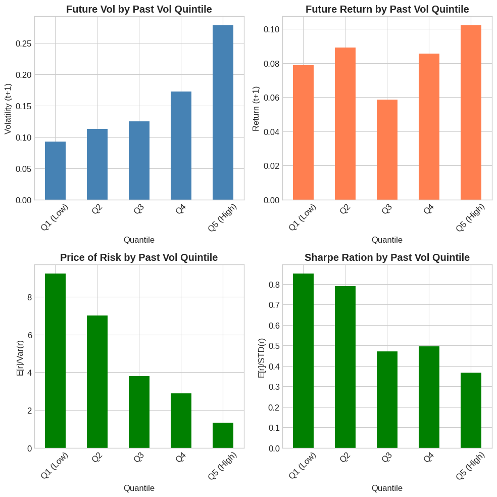
💡 Key Insight:
Returns are roughly flat across volatility quintiles, but volatility varies dramatically. This means the price of risk (return per unit variance) is much higher when volatility is low.
Strategy: Lever up when vol is low, reduce exposure when vol is high.
5.7.7. Building the Strategy #
5.7.7.1. From Signal to Weights#
The volatility-managed strategy uses weights:
where \(c\) is chosen so that the average weight equals 1:
# Compute weights
df['Weight_raw'] = 1 / df['RV_lag']
c = 1 / df['Weight_raw'].mean()
df['Weight'] = c * df['Weight_raw']

print(f"Scaling constant c: {c:.6f}")
print(f"Average weight: {df['Weight'].mean():.2f}")
Scaling constant c: 0.009079
Average weight: 1.00
# Visualize weights over time
fig, ax = plt.subplots(figsize=(12, 5))

ax.plot(df.index, df['Weight'], linewidth=0.8)
ax.axhline(1, color='red', linestyle='--', label='Buy & Hold (weight = 1)')

ax.set_xlabel('Date')
ax.set_ylabel('Weight on Market')
ax.set_title('Volatility-Managed Strategy Weights', fontsize=14, fontweight='bold')
ax.legend()

plt.tight_layout()
plt.show()
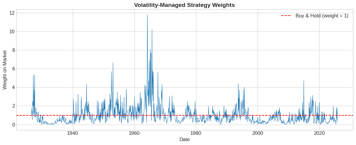
⚠️ Caution:
Leverage can get extreme! Weights can exceed 10x during calm periods. In practice, you’d want leverage limits.
5.7.7.2. Strategy Returns#
# Compute strategy returns
df['VMS'] = df['Weight'] * df['Mkt-RF']

# Cumulative returns comparison
fig, ax = plt.subplots(figsize=(12, 5))

cum_mkt = (1 + df['RF'] + df['Mkt-RF']).cumprod()
cum_vms = (1 + df['RF'] + df['VMS']).cumprod()

ax.plot(df.index, cum_mkt, label='Buy & Hold', linewidth=1.5)
ax.plot(df.index, cum_vms, label='Vol-Managed', linewidth=1.5)

ax.set_yscale('log')
ax.set_xlabel('Date')
ax.set_ylabel('Cumulative Return (log scale)')
ax.set_title('Volatility-Managed vs Buy & Hold', fontsize=14, fontweight='bold')
ax.legend()

plt.tight_layout()
plt.show()
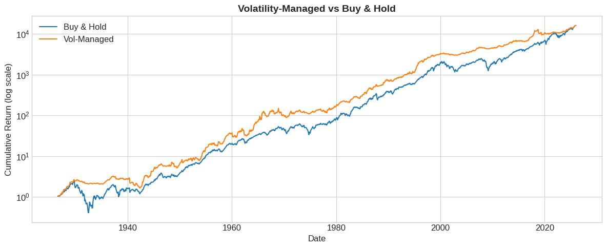
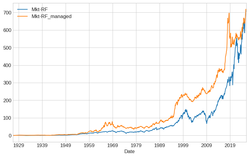
5.7.8. Performance Evaluation #
you end up in the same place. Does that mean that we didn’t accomplish anything?
Stear at the picture–what do you see?
5.7.8.2. Wrapping into a Function#
Let’s create a reusable function for volatility management:
def vol_managed_portfolio(factor_returns):
    """
    Construct a volatility-managed portfolio.

    Parameters:
    -----------
    factor_returns : pd.Series
        Daily factor returns
    max_leverage : float, optional
        Maximum allowed leverage (e.g., 3.0)

    Returns:
    --------
    df : DataFrame with returns and weights
    sr_managed : Sharpe ratio of managed strategy
    sr_unmanaged : Sharpe ratio of buy-and-hold
    """
    factor_name = factor_returns.name
    factor_returns = factor_returns.dropna()

    # Compute monthly realized variance
    end_of_month = factor_returns.index + pd.offsets.MonthEnd(0)
    RV = factor_returns.groupby(end_of_month).var() * 252

    # Aggregate to monthly returns
    monthly_ret = (1 + factor_returns).groupby(end_of_month).prod() - 1

    # Merge and lag
    df = pd.DataFrame({'RV': RV, factor_name: monthly_ret})
    df['RV_lag'] = df['RV'].shift(1)

    # Compute weights
    df['signal'] = 1 / df['RV_lag']
    df['Weight'] = df['signal'] / df['signal'].mean()


    # Compute managed returns
    df[f'{factor_name}_managed'] = df['Weight'] * df[factor_name]

    # Sharpe ratios
    sr_managed = (df[f'{factor_name}_managed'].mean() / df[f'{factor_name}_managed'].std()) * np.sqrt(12)
    sr_unmanaged = (df[factor_name].mean() / df[factor_name].std()) * np.sqrt(12)
    ((df[[factor_name,f'{factor_name}_managed']]+1).cumprod()-1).plot()
    return df, sr_managed, sr_unmanaged
# Test with leverage cap
df_factor_daily = get_factors('CAPM', freq='daily')
strategy_name='Mkt-RF'
# Without cap
df, sr_managed, sr_unmanaged = vol_managed_portfolio(df_factor_daily[strategy_name])
print(f"No leverage cap:")
print(f"  Unmanaged SR: {sr_unmanaged:.3f}")
print(f"  Managed SR:   {sr_managed:.3f}")
No leverage cap:
  Unmanaged SR: 0.452
  Managed SR:   0.520
5.7.9. Exercises #
5.7.9.1. 🔧 Exercise 1: Apply to all Factors in FF6#
Apply volatility timing to Mometum factor.
Load daily FF6 factor data
Run
vol_managed_portfolioon MOMCompare Sharpe ratio improvements
💡 Click for solution
df_ff = get_factors('FF6', freq='daily')

##Complete ___
for factor in ___:
    _, sr_m, sr_u = vol_managed_portfolio(df_ff[___])
    print(f"{factor}: Unmanaged = {sr_u:.3f}, Managed = {sr_m:.3f}, Δ = {sr_m - sr_u:.3f}")
# Your code here
5.7.9.2. 🔧 Exercise 2: Implement Leverage Limits#
Modify the function to cap leverage at different levels.
Test caps at 2x, 3x, 5x, and unlimited
Plot Sharpe ratio vs leverage cap
💡 Click for solution
caps = [2, 3, 5, 10, None]
srs = []


# You ahve to modify vol_managed_portfolio so this works
for cap in caps:
    _, sr, _ = vol_managed_portfolio(df_factor_daily['Mkt-RF'], max_leverage=cap)
    srs.append(sr)
    cap_str = str(cap) if cap else 'None'
    print(f"Cap = {cap_str}: SR = {sr:.3f}")

plt.figure(figsize=(8, 5))
plt.plot([str(c) if c else 'None' for c in caps], srs, 'o-')
plt.xlabel('Leverage Cap')
plt.ylabel('Sharpe Ratio')
plt.title('Sharpe Ratio vs Leverage Cap')
plt.show()
Higher caps allow more benefit but increase tail risk.
# Your code here
5.7.9.3. 🤔 Exercise 3: Volatility vs Variance Scaling#
If expected returns are proportional to volatility (not variance):
Recall optimal weights are
Then optimal weights are \(w_t \propto 1/\sigma_t\) instead of \(1/\sigma_t^2\).
Implement vol-scaling (use \(1/\sqrt{RV}\) instead of \(1/RV\))
Compare Sharpe ratios
Which works better for the market?
💡 Click for solution
# Variance scaling
df['Weight_var'] = 1 / df['RV_lag']
df['Weight_var'] /= df['Weight_var'].mean()

# Volatility scaling
df['Weight_vol'] = 1 / np.sqrt(df['RV_lag'])
df['Weight_vol'] /= df['Weight_vol'].mean()

# Compute returns
df['VMS_var'] = df['Weight_var'] * df['Mkt-RF']
df['VMS_vol'] = df['Weight_vol'] * df['Mkt-RF']

# Compare
sr_var = df['VMS_var'].mean() / df['VMS_var'].std() * np.sqrt(12)
sr_vol = df['VMS_vol'].mean() / df['VMS_vol'].std() * np.sqrt(12)

print(f"Variance scaling SR: {sr_var:.3f}")
print(f"Volatility scaling SR: {sr_vol:.3f}")
# Your code here
5.7.10. 📝 Key Takeaways #
Predicting variance is much easier than predicting returns. Past volatility strongly predicts future volatility.
If variance doesn’t predict returns, vol timing works. Invest more when vol is low, less when vol is high.
The price of risk declines with volatility. Average returns are roughly flat across vol regimes, so risk-adjusted returns are higher in calm periods.
Vol timing improves Sharpe ratios for most factors. This has been documented extensively since Moreira & Muir (2017).
Leverage can get extreme. Use caps or alternative scaling to keep positions reasonable.
Pod funds aggressively de-risk when vol spikes. If risk doesn’t predict returns, why take it?
Bonus question: What happens if everyone follows this advice? 🤔