Capital Allocation

8. Capital Allocation#

8.1. 🎯 Learning Objectives#

By the end of this notebook, you will be able to:

Formulate the capital allocation problem for an investor maximizing expected utility
Derive the mean-variance efficient (MVE) portfolio weights for risky assets
Understand the two-fund separation theorem and its practical implications
Explain how “all you need is Sharpe” simplifies portfolio construction
Implement alpha bets and portable alpha strategies in Python

#@title 🛠️ Setup: Run this cell first <a id="setup"></a>



import pandas as pd
import numpy as np
import matplotlib.pyplot as plt
import statsmodels.api as sm

%matplotlib inline

plt.style.use('seaborn-v0_8-whitegrid')
plt.rcParams['figure.figsize'] = [10, 6]

# Suppress warnings for cleaner output
import warnings
warnings.filterwarnings('ignore')

#@title 📦 Helper Function: get_factors()
import datetime
from pandas_datareader.data import DataReader
def get_factors(factors='CAPM', freq='daily'):
    """Download Fama-French factor data.

    Parameters:
    - factors: 'CAPM', 'FF3', 'FF5', or 'FF6'
    - freq: 'daily' or 'monthly'

    Returns: DataFrame with factor returns (as decimals)
    """
    freq_label = '' if freq == 'monthly' else '_' + freq

    if factors == 'CAPM':
        ff = DataReader(f"F-F_Research_Data_Factors{freq_label}", "famafrench", start="1921-01-01")
        df_factor = ff[0][['RF', 'Mkt-RF']]
    elif factors == 'FF3':
        ff = DataReader(f"F-F_Research_Data_Factors{freq_label}", "famafrench", start="1921-01-01")
        df_factor = ff[0][['RF', 'Mkt-RF', 'SMB', 'HML']]
    elif factors == 'FF5':
        ff = DataReader(f"F-F_Research_Data_Factors{freq_label}", "famafrench", start="1921-01-01")
        df_factor = ff[0][['RF', 'Mkt-RF', 'SMB', 'HML']]
        ff2 = DataReader(f"F-F_Research_Data_5_Factors_2x3{freq_label}", "famafrench", start="1921-01-01")
        df_factor = df_factor.merge(ff2[0][['RMW', 'CMA']], on='Date', how='outer')
    else:  # FF6
        ff = DataReader(f"F-F_Research_Data_Factors{freq_label}", "famafrench", start="1921-01-01")
        df_factor = ff[0][['RF', 'Mkt-RF', 'SMB', 'HML']]
        ff2 = DataReader(f"F-F_Research_Data_5_Factors_2x3{freq_label}", "famafrench", start="1921-01-01")
        df_factor = df_factor.merge(ff2[0][['RMW', 'CMA']], on='Date', how='outer')
        ff_mom = DataReader(f"F-F_Momentum_Factor{freq_label}", "famafrench", start="1921-01-01")
        df_factor = df_factor.merge(ff_mom[0], on='Date')
        df_factor.columns = ['RF', 'Mkt-RF', 'SMB', 'HML', 'RMW', 'CMA', 'MOM']

    if freq == 'monthly':
        df_factor.index = pd.to_datetime(df_factor.index.to_timestamp()) + pd.offsets.MonthEnd(0)
    else:
        df_factor.index = pd.to_datetime(df_factor.index)
    return df_factor / 100  # Convert from percent to decimal

8.3. The Capital Allocation Problem #

Every investor faces two fundamental questions:

How much risk should I take? (Allocation between risky and risk-free)
How should I spread that risk? (Allocation across risky assets)

💡 Key Insight:

A fundamental insight of portfolio theory is that these two decisions are separable:

First, find the portfolio with the best risk-return properties

Then, decide how much to allocate to it vs. the risk-free asset

8.3.1. Who Decides How Much Risk to Take?#

If you’re investing your own money (the principal), your optimal portfolio depends on:

Factor	Examples
Risk tolerance	How terrible you feel if you have less than expected
Investment horizon	Retirement in 5 years vs. 30 years
Financial goals	Minimum retirement income, college fund, property purchase
Background risk	Other income sources, job security

8.4. The Optimal Portfolio #

We model preferences using mean-variance utility:

\[\max_w \quad x \cdot E[r_p] - \frac{\gamma}{2} w^2 \cdot \text{Var}(r_p)\]

where:

$w$ = weight on the risky portfolio
$E[r_p]$ = expected excess return
$\gamma$ = risk aversion coefficient
$\text{Var}(r_p)$ = portfolio variance

Taking the derivative with respect to the weight and setting to zero:

\[w^* = \frac{1}{\gamma} \cdot \frac{E[r_p]}{\text{Var}(r_p)}\]

💡 Key Insight:

Your optimal weight is proportional to the risk-return trade-off.

Your optimal volatility is: $$w^* \cdot \sigma(r_p) = \frac{1}{\gamma} \cdot \text{Sharpe Ratio}$$

8.5. Factor Data #

We’ll work with the Fama-French 6 factors:

Factor	Description
Mkt-RF	Market excess return
SMB	Small minus Big (size)
HML	High minus Low (value)
RMW	Robust minus Weak (profitability)
CMA	Conservative minus Aggressive (investment)
MOM	Momentum

📌 How these factors are built:

All portfolios are market-cap-weighted: once we isolate the stocks for each side (long or short), we weight them by market cap

The long and short sides are the same size, so all these portfolios represent excess returns

Putting aside (very important) frictions in taking leverage, these portfolios are costless to implement—you fund your longs with your shorts

Except the market (where the short side is risk-free), all the others are designed to be market-neutral cross-sectional bets—you’re not taking a view on the market as a whole, only one segment against another

These portfolios are the core of the smart beta industry (also called systematic or quantitative investing)

Their construction has many details, which we will dig into in a later chapter

Players like Blackrock, AQR, Invesco, Dimensional Fund Advisors, Vanguard, and State Street make a living supplying these factors in easy-to-trade wrappers (ETFs or mutual funds)

# Load factor data
df = get_factors(factors='FF6', freq='monthly').dropna()

print(f"Data range: {df.index[0].strftime('%Y-%m')} to {df.index[-1].strftime('%Y-%m')}")
print(f"Number of months: {len(df)}")
df.head()

Data range: 1963-07 to 2025-12
Number of months: 750

	RF	Mkt-RF	SMB	HML	RMW	CMA	MOM
Date
1963-07-31	0.0027	-0.0039	-0.0057	-0.0081	0.0064	-0.0115	0.0101
1963-08-31	0.0025	0.0508	-0.0095	0.0170	0.0040	-0.0038	0.0100
1963-09-30	0.0027	-0.0157	-0.0025	0.0000	-0.0078	0.0015	0.0012
1963-10-31	0.0029	0.0254	-0.0057	-0.0004	0.0279	-0.0225	0.0313
1963-11-30	0.0027	-0.0086	-0.0116	0.0173	-0.0043	0.0227	-0.0078

# Separate risk-free and excess returns
rf = df['RF']
factors = df.drop(columns=['RF'])

# Summary statistics (annualized)
summary = pd.DataFrame({
    'Mean (ann.)': factors.mean() * 12,
    'Vol (ann.)': factors.std() * np.sqrt(12),
    'Sharpe': (factors.mean() * 12) / (factors.std() * np.sqrt(12)),
    'Freq 3 std dev':(factors.abs()/factors.std()>3).mean()
})
summary.round(3)

	Mean (ann.)	Vol (ann.)	Sharpe	Freq 3 std dev
Mkt-RF	0.071	0.154	0.462	0.008
SMB	0.017	0.105	0.166	0.008
HML	0.034	0.103	0.334	0.011
RMW	0.032	0.077	0.410	0.017
CMA	0.029	0.071	0.404	0.013
MOM	0.071	0.145	0.490	0.017

8.5.1. ⚡ In-Class Question: G1#

What is the optimal volatility for an investor who only invests in each of these assets individually? What is the optimal weight?
Pick an asset and show how the optimal portfolio variance changes as risk aversion $\gamma$ goes from close to zero (why not zero?) to very large (say 400)

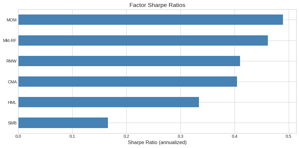
8.6. All You Need Is Sharpe? #

The Sharpe ratio is powerful because:

Higher SR → more growth per unit of risk
For the same growth, you need less risk
Higher expected growth → fewer large losses

⚠️ Caution:

Sharpe ratio is “all you need” only if:

You have mean-variance preferences

Returns are normally distributed

Normality

Always check the realized tails of your portfolio—are black swans too frequent?
How frequently 3 standard deviation events should be?

Preferences

do you care about all returns equally?
or is it more painfull to get a -20% returns in some situations? (we call “states of the world”)
What are examples of situations where would eb particularly bad for you to get a really bad return?
What about Bloomberg? Or Taylor Swift?

# Visualize the Sharpe ratios
fig, ax = plt.subplots(figsize=(10, 5))
summary['Sharpe'].sort_values().plot(kind='barh', ax=ax, color='steelblue')
ax.set_xlabel('Sharpe Ratio (annualized)', fontsize=12)
ax.set_title('Factor Sharpe Ratios', fontsize=14)
ax.axvline(x=0, color='black', linewidth=0.5)
plt.tight_layout()
plt.show()

../../_images/fad6477c8c683da81e40624bb1460c685318f92df73fb1e93984262f7e6dd76c.png

8.7. How do we combine these strategies?#

If I want the maximum return?
If I want the maximum Sharpe Ratio?
If I want the minimum Variance?
If I want the maximum return given a maximum desired variance?
If I want the minimum variance given a minimum desired return?

💡 What are the different approches we can take?

Pick the best asset for your criteria?
Grid of weights?
Solver?
Solve analytically

8.8. How do we combine these strategies? #

How do we build a portfolio that maximizes the mean-variance criteria?

\[ \max_W E[W'R^e]-\frac{\gamma}{2} Var(W'R^e)\]

How do we build a portfolio that maximizes the Expected excess return given a variance budget?

\[ \max_W E[W'R^e] \text{ subject to } Var(W'R^e)\leq \overline{V}\]

How do we build a portfolio that maximizes the Expected excess return?

\[ \max_W E[W'R^e]\]

How do we build a portfolio that minimizes Variance?

\[ \min_W Var[W'R^e]\]

How do we build a portfolio that maximizes Sharpe Ratio?

\[ \max_W \frac{E[W'R^e]}{\sqrt{Var[W'R^e]}}\]

💡 Key Insight:

The constrained problems (1, 2, and 3) all produce portfolios with the same relative weights—they all want the highest Sharpe ratio, but use it to achieve different goals!

⚡ In-Class Question: G4 — Explain in plain English what each of the five problems above is solving. Which ones have the same solution (up to scaling)?

8.8.1. Approaches#

Grid
Numerical
Math

What all these approaches require?

#@title 🛠️ Setup: Numerical Approach to portfolio maximization <a id="setup"></a>

# I implement maximum expected return given a variance buget
# it is easy to adjust to all other objectives
from scipy.optimize import minimize

def max_return_target_variance(mu_df, sigma_df, target_variance, options=None):
    """
    Solves for the maximum expected return portfolio given a cap on portfolio variance.

    Args:
        mu (pd.Series): Series of expected returns (N,).
        sigma_df (pd.DataFrame): Covariance matrix (N, N).
        target_variance (float): Maximum allowed portfolio variance.
        options (dict): Solver options (e.g., {'maxiter': 100, 'ftol': 1e-6}).

    Returns:
        pd.Series: Optimal weights for the portfolio (N,).
    """
    mu = mu_df.to_numpy()
    Sigma = sigma_df.to_numpy()
    num_assets = len(mu)

    # Objective function: minimize negative expected return to maximize expected return
    def objective(weights):
        return -np.dot(weights, mu)

    # Constraint 1: Sum of weights must be 1 (full investment)
    # Constraint 2: Portfolio variance must be less than or equal to target_variance
    # For 'ineq' constraints, the function must return a value >= 0.
    # So, target_variance - portfolio_variance >= 0
    #{'type': 'eq', 'fun': lambda weights: np.sum(weights) - 1}}
    constraints = [
        {'type': 'ineq',
        'fun': lambda weights: target_variance - np.dot(weights.T, np.dot(Sigma, weights))
    }]

    # Bounds for weights (assuming no short selling: 0 <= w_i <= 1)
    bounds = tuple((-10, 10) for _ in range(num_assets))

    # Initial guess (equal weights)
    initial_weights = np.array(num_assets * [1. / num_assets])



    # Solve the optimization problem using SLSQP (Sequential Least Squares Programming)
    result = minimize(
        objective,
        initial_weights,
        method='SLSQP',
        bounds=bounds,
        constraints=constraints,
        options=options
    )

    if result.success:
        return pd.Series(result.x, index=mu_df.index)
    else:
        raise ValueError(f"Optimization failed: {result.message}")

target_variance_monthly = 0.1**2/12
mu=factors.mean()
Sigma=factors.cov() # how do we estimate the variance-covariance matrix between the factors?

print("Solving for max return portfolio with variance cap...")
# Example: Setting max iterations and tolerance
#solver_options = {'maxiter': 1000, 'ftol': 1e-9}
solver_options = {}
optimal_weights_target_var = max_return_target_variance(mu, Sigma, target_variance_monthly, options=solver_options)

print("\nOptimal weights for max return with target variance cap:")
display(optimal_weights_target_var.round(4))

# Calculate portfolio statistics with the optimal weights
portfolio_return = np.dot(optimal_weights_target_var, mu)
portfolio_variance = np.dot(optimal_weights_target_var.T, np.dot(Sigma, optimal_weights_target_var))
portfolio_volatility = np.sqrt(portfolio_variance)

print(f"\nPortfolio Expected Monthly Return: {portfolio_return:.4f}")
print(f"Portfolio Monthly Variance: {portfolio_variance:.4f} (Target: <= {target_variance_monthly:.4f})")
print(f"Portfolio Monthly Volatility: {portfolio_volatility:.4f}")

print("\nAnnualized statistics:")
print(f"Portfolio Expected Annual Return: {portfolio_return * 12:.4f}")
print(f"Portfolio Annual Volatility: {portfolio_volatility * np.sqrt(12):.4f}")
print(f"Portfolio Annual SR: {portfolio_return/portfolio_volatility * np.sqrt(12):.4f}")

Solving for max return portfolio with variance cap...

Optimal weights for max return with target variance cap:

	0
Mkt-RF	0.5102
SMB	0.2480
HML	0.3379
RMW	0.3265
CMA	0.3123
MOM	0.5093

dtype: float64

Portfolio Expected Monthly Return: 0.0090
Portfolio Monthly Variance: 0.0008 (Target: <= 0.0008)
Portfolio Monthly Volatility: 0.0289

Annualized statistics:
Portfolio Expected Annual Return: 0.1077
Portfolio Annual Volatility: 0.1000
Portfolio Annual SR: 1.0767

8.9. The Math Approach #

\[ \max_W W'E[R^e]-\frac{\gamma}{2} W'Var(R^e) W\]

You find the maximum by differentiating with respect to the vector $W$ and setting to zero.

🤯 This is Calculus + Linear Algebra 🤯

The first order condition (optimality condition) is:

\[ E[R^e]-\gamma Var(R^e) W=0\]

👉 This is just saying that the marginal net benefit of investing more in any asset is exactly zero at the optimum.

Rearranging:

\[ E[R^e]=\gamma Var(R^e)W^*\]

Multiply both sides by the inverse of the covariance matrix:

\[ (\gamma Var(R^e))^{-1}E[R^e]=(\gamma Var(R^e))^{-1}\gamma Var(R^e)W^*\]

We get:

\[W^* = \frac{1}{\gamma} Var(R^e)^{-1} E[R^e]\]

where:

$E[R^e]$ is the vector of forward-looking expected excess returns
$Var(R^e)$ is the forward-looking variance-covariance matrix

💡 Key Insight:

This portfolio is the Holy Grail of quant investing 🤯

So simple, and yet so hard. Why? Because $E[R^e]$ and $Var(R^e)$ must be forward-looking estimates, and estimation is hard—especially for expected returns.

🐍 Python Insight: np.linalg.inv()

To compute the inverse of a matrix:
Sigma_inv = np.linalg.inv(Sigma)
For numerical stability with near-singular matrices, use:
Sigma_inv = np.linalg.pinv(Sigma)  # Pseudo-inverse
Inverse of matrix M is the matrix that the product produce the identity $M@M^{-1}=I$

For intution: for a scalar , $2*2^{-1}=1$, so $2^{-1}=1/2$

# Estimate moments from the sample
mu = factors.mean()  # Monthly expected returns
Sigma = factors.cov()  # Monthly covariance matrix

print("Expected excess returns (monthly):")
display(mu.round(4))
print("\nCovariance matrix:")
display(Sigma.round(6))

Expected excess returns (monthly):

	0
Mkt-RF	0.0059
SMB	0.0014
HML	0.0029
RMW	0.0026
CMA	0.0024
MOM	0.0059

dtype: float64

Covariance matrix:

	Mkt-RF	SMB	HML	RMW	CMA	MOM
Mkt-RF	0.001989	0.000396	-0.000274	-0.000188	-0.000325	-0.000321
SMB	0.000396	0.000913	-0.000128	-0.000270	-0.000105	-0.000067
HML	-0.000274	-0.000128	0.000883	0.000060	0.000418	-0.000243
RMW	-0.000188	-0.000270	0.000060	0.000494	0.000002	0.000075
CMA	-0.000325	-0.000105	0.000418	0.000002	0.000426	-0.000014
MOM	-0.000321	-0.000067	-0.000243	0.000075	-0.000014	0.001741

# Compute the MVE portfolio (unscaled)
Sigma_inv = np.linalg.inv(Sigma)
W_mve = Sigma_inv @ mu

print("MVE weights (unscaled):")
pd.Series(W_mve, index=factors.columns).round(2)

MVE weights (unscaled):

	0
Mkt-RF	5.58
SMB	3.23
HML	1.88
RMW	8.27
CMA	8.99
MOM	4.52

dtype: float64

8.9.1. ⚡ In-Class Question: G2#

Suppose you want to hit an expected excess return target of 5% per year. What is your optimal portfolio?

Hint: the final portfolio is $W^* = \lambda W_{MVE}$ where $\lambda$ is a scalar. What $\lambda$ do you need to achieve your goal?

# Compute MVE portfolio statistics
mve_return = W_mve @ mu  # Monthly
mve_var = W_mve @ Sigma @ W_mve  # Monthly
mve_vol = np.sqrt(mve_var)
mve_sharpe = (mve_return * 12) / (mve_vol * np.sqrt(12))

print(f"MVE Portfolio (annualized):")
print(f"  Expected return: {mve_return * 12:.2%}")
print(f"  Volatility: {mve_vol * np.sqrt(12):.2%}")
print(f"  Sharpe ratio: {mve_sharpe:.2f}")

MVE Portfolio (annualized):
  Expected return: 135.94%
  Volatility: 116.59%
  Sharpe ratio: 1.17

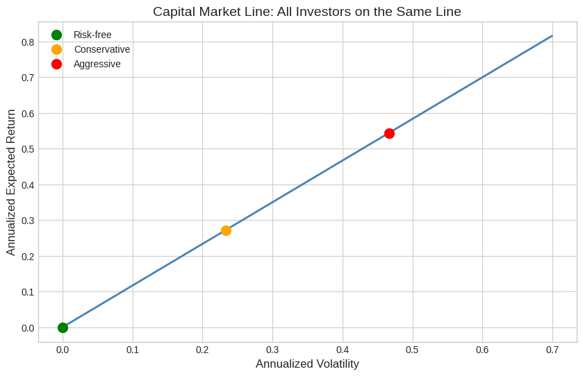
8.10. Two-Fund Separation #

The maximum Sharpe ratio portfolio is given by: $$W_{SR} = Var(R^e)^{-1} E[R^e]$$

This portfolio is also called:

MVE (Mean-Variance Efficient) portfolio (why?)
Tangency portfolio (why?)

💡 Key Insight: Leverage does not change Sharpe Ratio $$SR(lW'R)=\frac{lE[W'R]}{\sigma(lW'R)}=\frac{E[W'R]}{\sigma(W'R)}$$

This implies that if $W$ is MVE, $lW$ is also MVE for any l>0

💡 Key Insight: Two-Fund Separation

All investors—regardless of risk aversion—hold the same risky portfolio!

The scalar $\frac{1}{\gamma}$ just levers/delevers the portfolio.

Risk-averse investor: Small position in MVE + large position in risk-free

Risk-tolerant investor: Large (possibly leveraged) position in MVE

They differ only in how much, not what.

A risk-averse investor does not hold safer assets—it holds a safer portfolio that includes a little bit of the MVE portfolio and a lot of the risk-free asset.

A super risk-tolerant investor does not hold the riskiest assets—it holds a lot of the MVE portfolio, potentially leveraging its portfolio to get where it wants to be.

🤔 Think About It:

What does it mean that the relationship between expected return and volatility is linear along the Capital Market Line? Is that what you expect? Is that true in general as you change portfolio weights?

# Trace the investment frontier (Capital Market Line)
leverage_values = np.linspace(0, 0.6, 100)

frontier = []
for lev in leverage_values:
    W = lev * W_mve
    er = (W @ mu) * 12  # Annualized
    vol = np.sqrt(W @ Sigma @ W) * np.sqrt(12)  # Annualized
    frontier.append([lev, vol, er])

frontier = pd.DataFrame(frontier, columns=['Leverage', 'Volatility', 'Expected_Return'])

# Plot the Capital Market Line
fig, ax = plt.subplots(figsize=(10, 6))

ax.plot(frontier['Volatility'], frontier['Expected_Return'], linewidth=2, color='steelblue')
ax.scatter([0], [0], s=100, color='green', zorder=5, label='Risk-free')

# Mark some investor types
ax.scatter([frontier.iloc[33]['Volatility']], [frontier.iloc[33]['Expected_Return']],
           s=100, color='orange', zorder=5, label='Conservative')
ax.scatter([frontier.iloc[66]['Volatility']], [frontier.iloc[66]['Expected_Return']],
           s=100, color='red', zorder=5, label='Aggressive')

ax.set_xlabel('Annualized Volatility', fontsize=12)
ax.set_ylabel('Annualized Expected Return', fontsize=12)
ax.set_title('Capital Market Line: All Investors on the Same Line', fontsize=14)
ax.legend()
plt.show()

../../_images/14feb8d88d70a1e327ce72435465d16e064ea8df6fba2abebafb98a4854ecd6f.png

8.11. Alpha Bets and Portable Alpha #

It is useful to decompose your allocation into factor bets and alpha bets.

Most fund managers have tight limits on factor exposures, so factor exposure is more of a consequence of your alpha bets that you need to control rather than a form of active investing.

If you are a large capital allocator (pension fund, university endowment), then factor bets are also very important, since on average most of a portfolio’s risk is dominated by common factors.

Let’s say you identified N trading strategies:

Factor bets: Exposure to market, value, momentum, etc.
Alpha bets: Hedged positions with zero factor exposure

For alpha strategies with:

Alphas $\alpha$ (N×1)
Factor betas $\beta$ (N×1)
Idiosyncratic variance $\Sigma_\epsilon$

The optimal weights are:

\[W = \Sigma_\epsilon^{-1} \alpha\]

And the factor hedge:

\[W_f = -W'\beta\]

The factor hedge makes sure you have zero factor exposure in your portfolio.

8.11.1. When residuals are uncorrelated#

If the factors strip out all co-movement across strategies, $\Sigma_\epsilon$ is diagonal and we get a really clean formula:

\[\begin{split}\Sigma_{\epsilon}^{-1}\alpha=\left[\alpha_1,\alpha_2,...,\alpha_N\right]\left[\begin{array}{ccc}\sigma^2_{\epsilon,1} & 0 & 0\\0 & \sigma^2_{\epsilon,i} & 0\\0&0&\sigma^2_{\epsilon,N}\end{array}\right]^{-1}=\left[\begin{array}{c}\frac{\alpha_1}{\sigma^2_{\epsilon,1}} \\ \frac{\alpha_2}{\sigma^2_{\epsilon,2}} \\ \vdots \\ \frac{\alpha_N}{\sigma^2_{\epsilon,N}}\end{array}\right]\end{split}\]

The diagonal assumption leads to a really clean formula—but this is an assumption. What do we get in general?

8.11.2. Volatility allocations and the Appraisal Ratio#

Rewriting in terms of volatility allocations in each strategy:

\[W_i \sigma_{\epsilon,i} = \frac{\alpha_i}{\sigma_{\epsilon,i}}\]

What is this? Recall that the hedged portfolio return is:

\[r^e_i - \beta_i f = \alpha_i + \epsilon_i\]

so setting the hedge $h = -\beta_i$:

\[E[r^e_i - \beta_i f] = \alpha_i \quad \text{and} \quad \text{Var}(r^e_i - \beta_i f) = \sigma^2_{\epsilon,i}\]

So $\frac{\alpha_i}{\sigma_{\epsilon,i}}$ is the Sharpe ratio of the hedged strategy—i.e. the Appraisal Ratio.

🤔 Conceptual check: Suppose you have two assets and construct their hedged portfolios with respect to the market—what does the covariance of these hedged portfolios look like?

8.11.3. ⚡ In-Class Question: G3#

Scale the alpha portfolio weights to achieve a target volatility of 16% per year. What is $\lambda$?
What is your position on the market factor to maintain zero factor exposure?
Did we assume anything about the covariance matrix of the residuals, or did we let the data speak?
How would you impose that the covariance of the residuals are zero? Why would you?

# Estimate alpha and beta for each factor relative to the market
assets = ['SMB', 'HML', 'RMW', 'CMA', 'MOM']
market = 'Mkt-RF'

results = []
residuals_list = []
hedged_returns_list = []

for asset in assets:
    X = sm.add_constant(df[market])
    y = df[asset]
    model = sm.OLS(y, X).fit()

    results.append({
        'Asset': asset,
        'Alpha (ann.)': model.params['const'] * 12,
        'Beta': model.params[market],
        'Idio Vol (ann.)': model.resid.std() * np.sqrt(12)
    })
    residuals_list.append(model.resid)
    hedged_returns_list.append(model.params['const'] + model.resid)

results_df = pd.DataFrame(results).set_index('Asset')
residuals_matrix = np.vstack(residuals_list).T
hedged_returns_matrix = np.vstack(hedged_returns_list).T
Sigma_eps = np.cov(residuals_matrix.T)
results_df.round(3)

# Compute the optimal alpha portfolio
Alpha = results_df['Alpha (ann.)'].values / 12  # Convert back to monthly
residuals_matrix = np.vstack(residuals_list).T
Sigma_eps = np.cov(residuals_matrix.T)
print(Sigma_eps)
# Optimal weights
W_alpha = np.linalg.inv(Sigma_eps) @ Alpha

print("Optimal alpha portfolio weights (unscaled):")
pd.Series(W_alpha, index=assets).round(2)

[[ 8.34072612e-04 -7.37469815e-05 -2.32245941e-04 -4.03111675e-05
  -3.07030087e-06]
 [-7.37469815e-05  8.45190706e-04  3.36620086e-05  3.73289021e-04
  -2.87004006e-04]
 [-2.32245941e-04  3.36620086e-05  4.75828705e-04 -2.89123676e-05
   4.46110645e-05]
 [-4.03111675e-05  3.73289021e-04 -2.89123676e-05  3.72725440e-04
  -6.67099658e-05]
 [-3.07030087e-06 -2.87004006e-04  4.46110645e-05 -6.67099658e-05
   1.68943579e-03]]
Optimal alpha portfolio weights (unscaled):

	0
SMB	3.23
HML	1.88
RMW	8.27
CMA	8.99
MOM	4.52

dtype: float64

8.11.4. Combining the Hedged Portfolio (Alpha) and the Market (Beta)#

If your mandate allows and you see your factor investment as a purely financial decision—you care exclusively about the returns of the portfolio, not how the factor might co-move with your non-financial wealth—then combining the hedged portfolio with the market follows the same MVE logic.

But it is still useful to separate the two, as you probably have different confidence in the market risk premium than in the alphas.

The key insight is that the hedged portfolio has zero covariance with the market by construction—we took out any beta exposure!

\[\begin{split}Var(R^e)=\left[\begin{array}{cc} \sigma^2(R_{MKT}^e) & 0 \\ 0 & \sigma^2(R_{Hedged})\end{array}\right]\end{split}\]

So the optimal weights are simply:

\[\begin{split}W^* = \left[\begin{array}{c} \frac{E[R^e_{MKT}]}{\sigma^2(R_{MKT}^e)} \\ \frac{\alpha_{Hedged}}{\sigma^2(R_{Hedged})}\end{array}\right]\end{split}\]

👉 You invest in each strategy according to the strength of its risk-return trade-off.

8.11.5. From Individual Appraisals to Combined Sharpe Ratios#

For any two strategies A and B that have zero correlation with each other:

\[SR_{combined} = \sqrt{SR_{A}^2 + SR_{B}^2}\]

Since the hedged portfolio and the market are orthogonal by construction:

\[SR_{final} = \sqrt{SR_{MKT}^2 + SR_{Hedged}^2}\]

💡 Key Insight:

If you care about the SR of your final portfolio, you do not care about the SR of a particular strategy in isolation. You instead care about the SR of the strategy after you hedged out your current portfolio—i.e. the Appraisal Ratio. The appraisal ratio of each strategy relative to your portfolio is what actually matters.

# Compute hedged portfolio returns (alpha + residuals, not just residuals)
hedged_returns = hedged_returns_matrix @ W_alpha
hedged_er = hedged_returns.mean() * 12
hedged_vol = hedged_returns.std() * np.sqrt(12)
hedged_sr = hedged_er / hedged_vol

# Market stats
mkt_er = df[market].mean() * 12
mkt_vol = df[market].std() * np.sqrt(12)
mkt_sr = mkt_er / mkt_vol

# Combined
combined_sr = np.sqrt(mkt_sr**2 + hedged_sr**2)

print(f"Market Sharpe Ratio: {mkt_sr:.2f}")
print(f"Alpha Portfolio Sharpe (hedged): {hedged_sr:.2f}")
print(f"Combined Sharpe Ratio: {combined_sr:.2f}")

8.12. 📝 Exercises #

8.12.1. Exercise 1: Warm-up — Optimal Weight for a Single Asset#

🔧 Exercise:

For an investor with risk aversion $\gamma = 4$:

Compute the optimal weight for each factor individually

Compute the resulting portfolio volatility for each

Which factor would this investor allocate most to? Why?

# Your code here
gamma = 4

💡 Click to see solution

gamma = 4

for factor in factors.columns:
    mu_i = factors[factor].mean() * 12  # Annualized
    var_i = factors[factor].var() * 12  # Annualized
    
    x_star = (1 / gamma) * (mu_i / var_i)
    vol_port = abs(x_star) * factors[factor].std() * np.sqrt(12)
    
    print(f"{factor}: x* = {x_star:.2f}, Portfolio Vol = {vol_port:.2%}")

8.12.2. Exercise 2: Extension — Target Volatility Portfolio#

🤔 Think and Code:

You want a portfolio with 15% annualized volatility.

Find the leverage $\lambda$ to apply to the MVE portfolio

Compute the expected return at this volatility level

What weights result for each factor?

# Your code here
target_vol = 0.15

💡 Click to see solution

target_vol = 0.15

# Current MVE vol (annualized)
mve_vol_ann = mve_vol * np.sqrt(12)

# Leverage to hit target
leverage = target_vol / mve_vol_ann
print(f"Required leverage: {leverage:.2f}")

# Scaled weights
W_target = leverage * W_mve
print(f"\nTarget weights:")
print(pd.Series(W_target, index=factors.columns).round(2))

# Expected return
target_er = (W_target @ mu) * 12
print(f"\nExpected return at {target_vol:.0%} vol: {target_er:.2%}")

8.12.3. Exercise 3: Open-ended — Alpha + Beta Combination#

🤔 Think and Code:

You have an alpha portfolio (hedged) and the market:

What fraction of your risk budget should go to each?

Use the formula: allocate proportionally to $SR^2$

If you target 20% total volatility, what are the individual volatilities?

# Your code here

8.13. 🧠 Key Takeaways #

Separate the two decisions — First find the best risk-return portfolio, then decide how much risk to take
MVE portfolio formula: $W^* = \frac{1}{\gamma} \Sigma^{-1} E[R^e]$
Two-fund separation — All investors hold the same risky portfolio, just in different amounts
Portable alpha — Separate factor exposure from alpha by hedging out beta
Appraisal ratio matters — For adding to an existing portfolio, the hedged Sharpe ratio (appraisal ratio) is what counts

Concept	Formula
Optimal weight	$x^* = \frac{1}{\gamma} \frac{E[r]}{\text{Var}(r)}$
Optimal volatility	$x^* \sigma = \frac{SR}{\gamma}$
MVE weights	$W = \Sigma^{-1} E[R^e]$
Combined SR	$SR = \sqrt{SR_1^2 + SR_2^2}$ (if uncorrelated)

Concept	Formula
Optimal weight	\(x^* = \frac{1}{\gamma} \frac{E[r]}{\text{Var}(r)}\)
Optimal volatility	\(x^* \sigma = \frac{SR}{\gamma}\)
MVE weights	\(W = \Sigma^{-1} E[R^e]\)
Combined SR	\(SR = \sqrt{SR_1^2 + SR_2^2}\) (if uncorrelated)