
9. Cross-Sectional Trading strategies#
🎯 Learning Objectives
Contrast timing vs. cross-sectional approaches
Recognize that characteristic-based strategies keep aggregate market exposure roughly constant and instead shift weight across individual stocks according to firm-level signals.Master the four-step portfolio recipe
Build a signal → sort stocks each month → weight within buckets (equal or market-cap) → form the long-short spread (top – bottom), always using information that is known on the trade date.Construct the market-cap-weighted benchmark correctly
Compute market capitalizations from lagged price × shares-outstanding and show how to aggregate them to the total-market portfolio, avoiding look-ahead bias.Organize large equity data sets efficiently
Work with “stacked” (date-firm) data frames, merge CRSP returns with characteristics, and reshape the grouped returns so they are ready for analysis and plotting.Code a reusable function that maps any signal to portfolios
Generalize the recipe into a single function that takes a signal (X), number of groups, and weighting choice, and then delivers decile returns, cumulative-return plots, and the long-short series.Develop empirical intuition about trade-offs
Explore how the number of groups, the dispersion of the signal, and the choice of weights influence the return spread, volatility, and diversification of the resulting portfolios.
9.1. Libraries and all that#
# !pip install wrds
# import psycopg2
# import wrds
import pandas as pd
import numpy as np
import matplotlib.pyplot as plt
%matplotlib inline

import pandas_datareader.data as web

import datetime as dt

from dateutil.relativedelta import *
from pandas.tseries.offsets import *

def get_factors(factors='CAPM',freq='daily'):

    if freq=='monthly':
        freq_label=''
    else:
        freq_label='_'+freq


    if factors=='CAPM':
        fama_french = web.DataReader("F-F_Research_Data_Factors"+freq_label, "famafrench",start="1921-01-01")
        daily_data = fama_french[0]


        df_factor = daily_data[['RF','Mkt-RF']]
    elif factors=='FF3':
        fama_french = web.DataReader("F-F_Research_Data_Factors"+freq_label, "famafrench",start="1921-01-01")
        daily_data = fama_french[0]

        df_factor = daily_data[['RF','Mkt-RF','SMB','HML']]
    elif factors=='FF5':

        fama_french = web.DataReader("F-F_Research_Data_Factors"+freq_label, "famafrench",start="1921-01-01")
        daily_data = fama_french[0]

        df_factor = daily_data[['RF','Mkt-RF','SMB','HML']]
        fama_french2 = web.DataReader("F-F_Research_Data_5_Factors_2x3"+freq_label, "famafrench",start="1921-01-01")
        daily_data2 = fama_french2[0]

        df_factor2 = daily_data2[['RMW','CMA']]
        df_factor=df_factor.merge(df_factor2,on='Date',how='outer')

    else:
        fama_french = web.DataReader("F-F_Research_Data_Factors"+freq_label, "famafrench",start="1921-01-01")
        daily_data = fama_french[0]

        df_factor = daily_data[['RF','Mkt-RF','SMB','HML']]
        fama_french2 = web.DataReader("F-F_Research_Data_5_Factors_2x3"+freq_label, "famafrench",start="1921-01-01")
        daily_data2 = fama_french2[0]

        df_factor2 = daily_data2[['RMW','CMA']]
        df_factor=df_factor.merge(df_factor2,on='Date',how='outer')
        fama_french = web.DataReader("F-F_Momentum_Factor"+freq_label, "famafrench",start="1921-01-01")
        df_factor=df_factor.merge(fama_french[0],on='Date')
        df_factor.columns=['RF','Mkt-RF','SMB','HML','RMW','CMA','MOM']
    if freq=='monthly':
        df_factor.index = pd.to_datetime(df_factor.index.to_timestamp())
    else:
        df_factor.index = pd.to_datetime(df_factor.index)


    return df_factor/100
9.2. The Market-Cap Weighted strategy#
As a warm up for you first factor construction we will construct the returns on the market portfolio
In some way that is the most important strategy ever
It completely revolutionized Wall Street leading to the rise of index funds
How to do it?
start with a vector of market capitalization for all relevant assets \(M_t=[m_t^{AAPL},m_t^{GOOG},m_t^{TSLA},..]\)
The strategy then set the weights simply to
So at end of month t you look at the market caps, construct the weights, and buy the assets with weights \(X_t\) (at prices \(P_t\)) to earn
at the end of the next month.
That is you pay \(P_t\) and get back \(P_{t+1}+D_{t+1}\), hence return \(R_{t+1}=\frac{P_{t+1}+D_{t+1}}{P_t}\)
This portfolio has nice properties
This portfolio is very easy to trade. It does not require re-balancing as your weights naturally go up if the stock rallies and go down if the stock crashes
You can implement this approach to any subset of firms (for example SP500 or Russel2000) are market cap indexes that track a particular universe of stocks and we will be using it in our characteristic-based portfolios shortly
By buying proportionally to market cap you never have to build a huge position in a tiny stock–so this is much easier to trade!
Equal weighted portfolio tend to be very hard to trade and the alphas that you get there are mostly a mirrage, unless you focus on large caps
Steps
Get firm level monthly return data with market capitalizations
clean up/organize the data set
Make sure to lag the market cap signal so that we use prices from last month to trade at the start of this month ( we could also skip another month to be extra sure)
Construct the weighted average of returns across stocks for each date
9.2.1. Stacked Datasets#
We will now work with large data sets
Data sets that include all US stocks
Because there are many stocks, we have to work with it stacked
Organizing the data
The objective here is to have a data set with
Security identifier
Date of the information
Monthly return of the firm in that month
Market capitalization of the firm in that month
########################
### Download CRSP monthly data
###################
# conn=wrds.Connection()
# crsp = conn.raw_sql("""
#                       select a.permno,a.permco, a.date, b.shrcd, b.exchcd,b.ticker,
#                       a.ret, a.shrout, a.prc,a.retx
#                       from crsp.msf as a
#                       left join crsp.msenames as b
#                       on a.permno=b.permno
#                       and b.namedt<=a.date
#                       and a.date<=b.nameendt
#                       where a.date between '01/31/2002' and '12/31/2024'
#                       and b.exchcd between 1 and 3
#                       and b.shrcd between 10 and 11
#                       """, date_cols=['date'])

# crsp.to_pickle('../../assets/data/crspm2002_2024.pkl')
# # variables downloaded
# # 1. Permno-- are unique indentifier to a security
# # (for exmaple a stock that has multiple types of stocks will have multiple permnos)

# # 2. shrco is the type of share: common share, ADR, ETF, ....
# # we will focus on common shares

# # 3. exchcd is the code of the exchange where the stock was originally listed
# # we will focus on stock listed in the 3 major stock exchanges ( basically the whole market)

# # 4. ret,retx, shrout,  prc, are the stock return, the stock return excluding dividends, number of shares outstanding, and price

# # 5. date is the trading date of the return

#####
# get pre downloaded data

url = "https://github.com/amoreira2/UG54/blob/main/assets/data/crspm2002_2024.pkl?raw=true"
crsp = pd.read_pickle(url)
crsp
| permno | permco | date | shrcd | exchcd | ticker | ret | shrout | prc | retx | |
|---|---|---|---|---|---|---|---|---|---|---|
| 0 | 10066 | 6331 | 2002-02-28 | 11 | 2 | FCM | -0.333333 | 43809.0 | 0.040 | -0.333333 |
| 1 | 10066 | 6331 | 2002-03-28 | 11 | 2 | FCM | 0.000000 | 43809.0 | 0.040 | 0.000000 |
| 2 | 10066 | 6331 | 2002-04-30 | 11 | 2 | FCM | -0.250000 | 43809.0 | 0.030 | -0.250000 |
| 3 | 10066 | 6331 | 2002-05-31 | 11 | 2 | FCM | 0.333333 | 43809.0 | 0.040 | 0.333333 |
| 4 | 10066 | 6331 | 2002-06-28 | 11 | 2 | FCM | -0.250000 | 43809.0 | 0.030 | -0.250000 |
| ... | ... | ... | ... | ... | ... | ... | ... | ... | ... | ... |
| 144996 | 78830 | 11893 | 2006-06-30 | 11 | 3 | TRUE | -0.048387 | 2263.0 | -23.010 | -0.048387 |
| 144997 | 78830 | 11893 | 2006-07-31 | 11 | 3 | TRUE | 0.030204 | 2263.0 | -23.705 | 0.030204 |
| 144998 | 78830 | 11893 | 2006-08-31 | 11 | 3 | TRUE | -0.031850 | 2233.0 | 22.950 | -0.031850 |
| 144999 | 78830 | 11893 | 2006-09-29 | 11 | 3 | TRUE | 0.006972 | 2233.0 | 23.110 | 0.006972 |
| 145000 | 78830 | 11893 | 2006-10-31 | 11 | 3 | TRUE | -0.026396 | 2233.0 | 22.500 | -0.026396 |
1145001 rows × 10 columns
9.3. Data Cleaning and Organization#
crsp=crsp[['permco','permno','ticker','date','ret','shrout','prc']].copy()
# change variable format to int
crsp[['permno']]=crsp[['permno']].astype(int)

# Line up date to be end of month
crsp['date']=crsp['date']+pd.offsets.MonthEnd(0)

# calculate market equity
# why do we use absolute value of price?
crsp['me']=crsp['prc'].abs()*crsp['shrout']

# sort by permno and date and also drop duplicates
crsp=crsp.sort_values(by=['permno','date']).drop_duplicates()

crsp
| permco | permno | ticker | date | ret | shrout | prc | me | |
|---|---|---|---|---|---|---|---|---|
| 212 | 7953 | 10001 | EWST | 2002-01-31 | -0.013100 | 2566.0 | 11.30000 | 2.899580e+04 |
| 213 | 7953 | 10001 | EWST | 2002-02-28 | -0.053097 | 2569.0 | 10.70000 | 2.748830e+04 |
| 214 | 7953 | 10001 | EWST | 2002-03-31 | -0.015888 | 2571.0 | 10.40000 | 2.673840e+04 |
| 215 | 7953 | 10001 | EWST | 2002-04-30 | -0.043269 | 2571.0 | 9.95000 | 2.558145e+04 |
| 216 | 7953 | 10001 | EWST | 2002-05-31 | 0.014824 | 2571.0 | 10.09750 | 2.596067e+04 |
| ... | ... | ... | ... | ... | ... | ... | ... | ... |
| 144132 | 53453 | 93436 | TSLA | 2024-08-31 | -0.077391 | 3194640.0 | 214.11000 | 6.840044e+08 |
| 144133 | 53453 | 93436 | TSLA | 2024-09-30 | 0.221942 | 3207000.0 | 261.63000 | 8.390474e+08 |
| 144134 | 53453 | 93436 | TSLA | 2024-10-31 | -0.045025 | 3210060.0 | 249.85001 | 8.020335e+08 |
| 144135 | 53453 | 93436 | TSLA | 2024-11-30 | 0.381469 | 3210060.0 | 345.16000 | 1.107984e+09 |
| 144136 | 53453 | 93436 | TSLA | 2024-12-31 | 0.170008 | 3210060.0 | 403.84000 | 1.296351e+09 |
1145001 rows × 8 columns
from pandas.tseries.offsets import *
crsp=crsp[['permco','permno','ticker','date','ret','shrout','prc']].copy()
# change variable format to int
crsp[['permno']]=crsp[['permno']].astype(int)
crsp[['permco']]=crsp[['permco']].astype(int)
# Line up date to be end of month
crsp['date']=crsp['date']+MonthEnd(0)

# calculate market equity
# why do we use absolute value of price?
crsp['me']=crsp['prc'].abs()*crsp['shrout']
# drop price and shareoustandng since we won't need it anymore
crsp=crsp.drop(['prc','shrout'], axis=1)
crsp_me=crsp.groupby(['date','permco'])['me'].sum().reset_index()


# largest mktcap within a permco/date
crsp_maxme = crsp.groupby(['date','permco'])['me'].max().reset_index()

# join by jdate/maxme to find the permno
crsp=pd.merge(crsp, crsp_maxme, how='inner', on=['date','permco','me'])

# drop me column and replace with the sum me
crsp=crsp.drop(['me'], axis=1)

# join with sum of me to get the correct market cap info
crsp=pd.merge(crsp, crsp_me, how='inner', on=['date','permco'])

# sort by permno and date and also drop duplicates
crsp=crsp.sort_values(by=['permno','date']).drop_duplicates()
9.4. Stacked Datasets structure#
Take time to note the stacked structure of the data set
Before with a “rectangular” data set we need two coordinates, row and column, to identify the return of an asset in a particular date
It was easier to manipulate but we would need one dataframe for each different firm variable: In this case one for return and one for market equity
As we work with many signals, this becomes intractable because we would need many dataframes
As we work with many asset, this would become intractable because we would need dataframes with many columns with most locations empty. This is very inefficient and hard to manipulate
Now we need two coordinates both in columns, “date” and “permco”, to identify one firm-date observation, and then a third coordinate, the column names to identify the particular variable for that firm-date pair
crsp.head()
| permco | permno | ticker | date | ret | me | |
|---|---|---|---|---|---|---|
| 0 | 7953 | 10001 | EWST | 2002-01-31 | -0.013100 | 28995.8000 |
| 1 | 7953 | 10001 | EWST | 2002-02-28 | -0.053097 | 27488.3000 |
| 2 | 7953 | 10001 | EWST | 2002-03-31 | -0.015888 | 26738.4000 |
| 3 | 7953 | 10001 | EWST | 2002-04-30 | -0.043269 | 25581.4500 |
| 4 | 7953 | 10001 | EWST | 2002-05-31 | 0.014824 | 25960.6725 |
9.5. constructing portfolio weights#
We are constructing a market capitalization weighted strategy
It is key that the weights are know at the time of portfolio formation
So we need to lag our portfolio weights
Lagging the market cap signal
We use the method
.shift(d)which “lags” the data by d periods.It is important that we have our data set sorted by date
shift(d)simply shifts the rows. So you have to make sure that it is actually lagging by date. The way to do that is togroupbysecurity and applying the shift within security.
Why this is important?
Because the data set is stacked so when you shift the first month of security n, it will end up returning the last month of security n-1.
By “grouping by” we correctly assign a missing value there since we don’t have the data
# sort by permno and date and set as index
crsp=crsp.sort_values(by=['permno','date'])
crsp['me_l1']=crsp.groupby(['permno']).me.shift(1)
crsp
| permco | permno | ticker | date | ret | me | me_l1 | |
|---|---|---|---|---|---|---|---|
| 0 | 7953 | 10001 | EWST | 2002-01-31 | -0.013100 | 2.899580e+04 | NaN |
| 1 | 7953 | 10001 | EWST | 2002-02-28 | -0.053097 | 2.748830e+04 | 2.899580e+04 |
| 2 | 7953 | 10001 | EWST | 2002-03-31 | -0.015888 | 2.673840e+04 | 2.748830e+04 |
| 3 | 7953 | 10001 | EWST | 2002-04-30 | -0.043269 | 2.558145e+04 | 2.673840e+04 |
| 4 | 7953 | 10001 | EWST | 2002-05-31 | 0.014824 | 2.596067e+04 | 2.558145e+04 |
| ... | ... | ... | ... | ... | ... | ... | ... |
| 1130765 | 53453 | 93436 | TSLA | 2024-08-31 | -0.077391 | 6.840044e+08 | 7.413801e+08 |
| 1130766 | 53453 | 93436 | TSLA | 2024-09-30 | 0.221942 | 8.390474e+08 | 6.840044e+08 |
| 1130767 | 53453 | 93436 | TSLA | 2024-10-31 | -0.045025 | 8.020335e+08 | 8.390474e+08 |
| 1130768 | 53453 | 93436 | TSLA | 2024-11-30 | 0.381469 | 1.107984e+09 | 8.020335e+08 |
| 1130769 | 53453 | 93436 | TSLA | 2024-12-31 | 0.170008 | 1.296351e+09 | 1.107984e+09 |
1130770 rows × 7 columns
9.6. Portfolio Weights#
We now want to compute the returns of our portfolio
We need to start with the weights
Question
Write the code that constructs the vector of weights for the date ‘2015-06-60’
Write the core that returns that the portfolio return in data date
# _temp=crsp[____==___]
# W=_temp[]/(_temp[___].___)
# _temp[___]@W
9.7. Portfolio returns#
def portreturn(x):
    return (x['me_l1']*x['ret']/x['me_l1'].sum()).sum()

#try first if it works in one date
_temp=crsp[crsp.date=='2015-06-30']
portreturn(_temp)

# no apply to all dates
Rmkt=crsp.groupby(['date']).apply(portreturn)

#try first if it works in one date

portreturn(_temp)

# no apply to all dates
Rmkt=crsp.groupby(['date']).apply(portreturn)
/var/folders/ft/hpl8ntq506jgz116vbqnwqj40000gp/T/ipykernel_24224/3402911068.py:9: DeprecationWarning: DataFrameGroupBy.apply operated on the grouping columns. This behavior is deprecated, and in a future version of pandas the grouping columns will be excluded from the operation. Either pass `include_groups=False` to exclude the groupings or explicitly select the grouping columns after groupby to silence this warning.
  Rmkt=crsp.groupby(['date']).apply(portreturn)
/var/folders/ft/hpl8ntq506jgz116vbqnwqj40000gp/T/ipykernel_24224/3402911068.py:16: DeprecationWarning: DataFrameGroupBy.apply operated on the grouping columns. This behavior is deprecated, and in a future version of pandas the grouping columns will be excluded from the operation. Either pass `include_groups=False` to exclude the groupings or explicitly select the grouping columns after groupby to silence this warning.
  Rmkt=crsp.groupby(['date']).apply(portreturn)
What is the code that does each step?
The
Xmethod groups the data by month so we obtain the return of the portfolio in that monththe code
Yhas the weights in a given date, which for each date will return a vector that adds up to one.the code
Zmultiplies the return of each asset by the weightthe code
Wsum all up to get the return of the portfolio
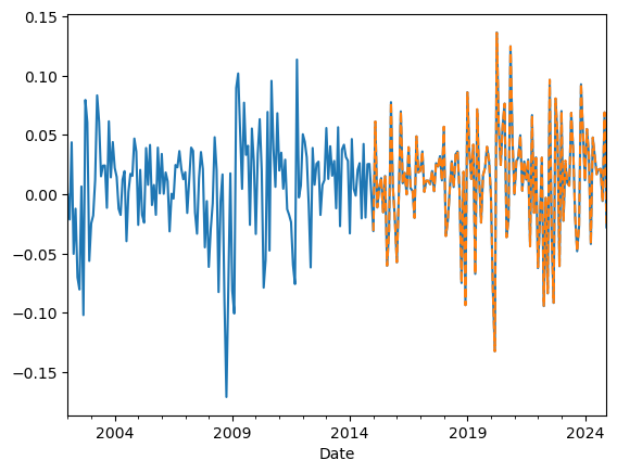
Lets compare our factor with the one ken french website
#Lets look at the cumulative return
df=get_factors('CAPM',freq='monthly')
(Rmkt).plot()
(df['Mkt-RF']+df['RF'])['2015':'2024'].plot(linestyle='dashed')
/var/folders/ft/hpl8ntq506jgz116vbqnwqj40000gp/T/ipykernel_24224/1743910507.py:22: FutureWarning: The argument 'date_parser' is deprecated and will be removed in a future version. Please use 'date_format' instead, or read your data in as 'object' dtype and then call 'to_datetime'.
  fama_french = web.DataReader("F-F_Research_Data_Factors"+freq_label, "famafrench",start="1921-01-01")
<Axes: xlabel='Date'>
Things to try and think about
Suppose you lag market cap 2 months instead of 1 does it make any difference? Do you expect there is any difference
Suppose you drop the stocks with “negative” prices (i.e. stocks that didn’t trade in the last day of the month), do you expect any difference? Does it make a difference?
I want everyone to stop and think about how one would approach the problem below. Please chat with your group!
Harder: Suppose you wanted to construct something “like” the SP500? I.e. do market cap weights but only for the 500 largest firms in a given month. How would you do that?
9.8. Characteristic-Based Strategies#
So far we have looked at strategies that go in and out of a particular asset according to a signal.
Now we will look at strategies that trade on asset characteristics
The recipe
Construct a characteristic for each stock.
It can be based on accounting data (aka fundamentals), return data, textual data from earning calls, twitter activity, ownership, shorting activity, satellite images–ANYTHING
What is important is that for each stock in each date you have a value for this characteristic
This characteristic must vary across firms
And you have a sense/theory of how this characteristic relates to expected returns
On a given date sort stocks by this characteristic.
It is key that this characteristic is in fact known at sorting date!
Extremely careful not to introduce “look-ahead” bias
Construct portfolios by dividing stocks in deciles/quintiles to form portfolios of stocks that have similar characteristic
You can either equal-weight or value-weight or volume-weights or signal-weight within portfolio
Value-weighed portfolios are easier to trade, but if you are focused on large caps, you can go with either
But what is important is that each portfolio will have stocks of have very different characteristic values
Construct the long-short where you go long portfolio “10” and short portfolio “1” (or vice versa) but the point is to take a bet on the characteristic spread
The goal here is to produce Alpha
this is a simple and algorithimic way to implement your idea in a way that harvest the benefits of diversification
Instead of betting on Apple because it is exposed to tariffs, build a tariff exposure “characteristic”
From “names” to characteristics
The sorting by date keeps the stocks inside the portfolios with similar characteristics
This sorting will “work” if these characteristics are good proxies for the behavior of the stock returns
Indeed, the key is that each portfolio has stocks of vastly different characterisitcs and keeps churning as firms change
Let’s take MSFT (microsoft) as an example:
MSFT transitioned from being small in the 80’s to be gigantic in the 90’s, as a result, it moved up from the small portfolio to the big portfolio
During the Tech boom when MSFT had a huge valuation relative to it’s book value, it went to the low BM portfolio
But then MSFT transtioned back to the high BM portfolio once it’s market valuation collapsed in the aftermath of the techbubble
Now with AI, MSFT is back into the low BM portfolio
During these 80 years MSFT changed dramatically and the characteristic changed with it…
The key is that firms’ characteristics change over time, by constructing portfolios, we hope to estimate some stable parameters (for example, alpha and beta)
But it doesn’t work always, if you use the first letter of stock ticker to construct 26 portfolios you are unlikely to get spread in average returns and most likely each portfolio will resemble the market portfolio but with much more volatility.
The characteristics have to capture the right economics/market dynamics
9.9. Implementing the recipe#
We will start with a constructed characteristic \(c_{i,t}\)
Produce 10 portfolios based on this characteristic
Members of portfolio 1 in date t have the bottom 10% value of the characteristics in date t
Members of portfolio 2 in date t have characteristic between 10% and 20% of the characteristics in date t
Given these memberships for each date we will the construct return by buying at the closing price of date t and selling at the closing on date t+1
We will typically work with monthly data, so this should read as the closing of the last date of months t and t+1
We start by loading a dataset where you have many signals
9.10. Our Characteristic data#
They are based on various accounting and market based information
The construction of each signal is full of painful details and there are many details that matter
Here are some of the variables
permno identifies the company in a way that is invariant to ticker changes
re is the excess return on the stock
rme is the market excess returns ( the same across all stocks in a given date)
rf is the risk-free rate (also the same across stocks)
size is log market cap
Value is Book-to-market (Why is this called value?)
There are many other characteristics
For now all we need to know is that all the characteristics are already lagged 1 month, so we can form portfolios directly based on them without lagging
url = "https://github.com/amoreira2/UG54/blob/main/assets/data/characteristics20022016.pkl?raw=true"

df_X = pd.read_pickle(url)
df_X=df_X.reset_index()
df_X.date=df_X.date+pd.tseries.offsets.MonthEnd()
df_X.info()
<class 'pandas.core.frame.DataFrame'>
RangeIndex: 163913 entries, 0 to 163912
Data columns (total 34 columns):
 #   Column     Non-Null Count   Dtype
---  ------     --------------   -----
 0   date       163913 non-null  datetime64[ns]
 1   permno     163913 non-null  int64
 2   re         163913 non-null  float64
 3   rf         163913 non-null  float64
 4   rme        163913 non-null  float64
 5   size       163913 non-null  float64
 6   value      163913 non-null  float64
 7   prof       163913 non-null  float64
 8   fscore     163913 non-null  int64
 9   debtiss    163913 non-null  int64
 10  repurch    163913 non-null  int64
 11  nissa      163913 non-null  float64
 12  growth     163913 non-null  float64
 13  aturnover  163913 non-null  float64
 14  gmargins   163913 non-null  float64
 15  ep         163913 non-null  float64
 16  sgrowth    163913 non-null  float64
 17  lev        163913 non-null  float64
 18  roaa       163913 non-null  float64
 19  roea       163913 non-null  float64
 20  sp         163913 non-null  float64
 21  mom        163913 non-null  float64
 22  indmom     163913 non-null  int64
 23  mom12      163913 non-null  float64
 24  momrev     163913 non-null  float64
 25  valuem     163913 non-null  float64
 26  nissm      163913 non-null  float64
 27  strev      163913 non-null  float64
 28  ivol       163913 non-null  float64
 29  betaarb    163913 non-null  float64
 30  indrrev    163913 non-null  float64
 31  price      163913 non-null  float64
 32  age        163913 non-null  float64
 33  shvol      163913 non-null  float64
dtypes: datetime64[ns](1), float64(28), int64(5)
memory usage: 42.5 MB
9.11. Group assets by signal#
Select our characteristic
assign stocks to groups. These groups will identify which portfolio each stock belongs in a particular date according to their relative ranking of the characteristic in that date
We will do this by applying the function pd.qcut to the chosen characteristic. This will “cut” the signal distribution in the chosen number of groups.
The important aspects is that we will be applying this date by date. This make the strategy cross-sectional because you are using the distribution of the signal as given date to do the grouping– Very much like curved grades by cohort
Details
duplicates='drop': In case there are two stocks with exactly the same signal that are exactly in the cutoff of the groups, we drop one of the observationslabels=False: The method simply label the groups with numbers. For example ifngroups=10then it will assign0to the stocks with the bottom 10% returns in a given date,1to stocks with returns in between 10% and 20% of the signal distribution on a given date, …, and 9 for stocks in the top 10% (signal in between 90% and 100% of the return distribution on a given date) .
group='value'
df_X['X_group']=df_X.groupby(['date'])[group].transform(lambda x: pd.qcut(x, 10, labels=False,duplicates='drop'))
df_X[['date','permno',group,'X_group']]
| date | permno | value | X_group | |
|---|---|---|---|---|
| 0 | 2002-01-31 | 10078 | -2.471709 | 0 |
| 1 | 2002-01-31 | 10104 | -3.183480 | 0 |
| 2 | 2002-01-31 | 10107 | -1.696643 | 2 |
| 3 | 2002-01-31 | 10108 | -1.461118 | 3 |
| 4 | 2002-01-31 | 10119 | -0.521094 | 7 |
| ... | ... | ... | ... | ... |
| 163908 | 2016-12-31 | 93420 | 1.049163 | 9 |
| 163909 | 2016-12-31 | 93422 | 0.829353 | 9 |
| 163910 | 2016-12-31 | 93423 | -2.128977 | 1 |
| 163911 | 2016-12-31 | 93429 | -3.001095 | 0 |
| 163912 | 2016-12-31 | 93436 | -3.328269 | 0 |
163913 rows × 4 columns
9.12. Calculate the portfolio return#
We need weights where they must add up to 1.
We do this so when we do the long-short we have a clear notion of “book size”
if you go 100 times the long short, you know this means buy 100 dollars of the long and selling 100 dollars of the short
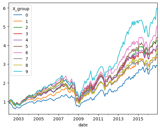
We will start with equal-weighted returns which is easy and it is simply an average of the returns in the portfolio in a given date ( the wrights is 1/I)
⚡ ⏰ Question: Group F-G ⚡
Complete the code below so we obtain the output below with the cumulative returns for each portfolio
# Calculate the equal-weighted portfolio returns for each date and group
ret_byX_ew = df_X.groupby(['date','X_group']).apply(lambda x: np.mean(x['re'] + x['rf']))
# what this code below does?
ret_byX_ew = ret_byX_ew.unstack(level=-1)

(ret_byX_ew + 1).cumprod().plot()
/var/folders/ft/hpl8ntq506jgz116vbqnwqj40000gp/T/ipykernel_24224/1988538451.py:2: DeprecationWarning: DataFrameGroupBy.apply operated on the grouping columns. This behavior is deprecated, and in a future version of pandas the grouping columns will be excluded from the operation. Either pass `include_groups=False` to exclude the groupings or explicitly select the grouping columns after groupby to silence this warning.
  ret_byX_ew = df_X.groupby(['date','X_group']).apply(lambda x: np.mean(x['re'] + x['rf']))
<Axes: xlabel='date'>
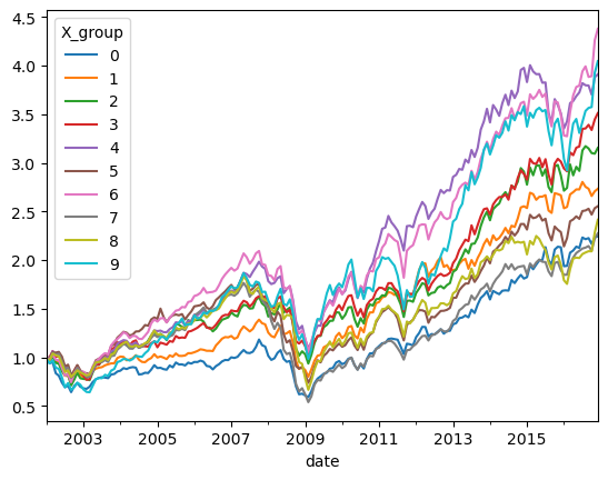
9.13. Market cap weighted returns#
What about for market cap weights?
df_X['me_l1']=np.exp(df_X['size'])
ret_byX_vw =df_X.groupby(['date','X_group']).apply(lambda x:((x['re']+x['rf'])*x['me_l1']).sum()/(x['me_l1'].sum()))
ret_byX_vw=ret_byX_vw.unstack(level=-1)
(ret_byX_vw+1).cumprod().plot()
/var/folders/ft/hpl8ntq506jgz116vbqnwqj40000gp/T/ipykernel_24224/1411861043.py:2: DeprecationWarning: DataFrameGroupBy.apply operated on the grouping columns. This behavior is deprecated, and in a future version of pandas the grouping columns will be excluded from the operation. Either pass `include_groups=False` to exclude the groupings or explicitly select the grouping columns after groupby to silence this warning.
  ret_byX_vw =df_X.groupby(['date','X_group']).apply(lambda x:((x['re']+x['rf'])*x['me_l1']).sum()/(x['me_l1'].sum()))
<Axes: xlabel='date'>
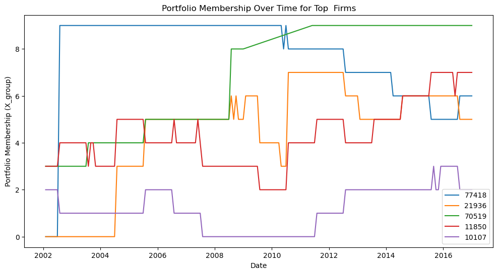
9.14. The evolution of a firm through the lens of a characteristic#
-If we focus on a particular stock, we can see how it’s portfolio membership changed over time.
-You can check you that some characteristics are fairly persistent and change only slowly over time
-While others, like momentum change very frequently.
We will look at the 5 largest firms as of 2002
I did a query to get their tickers so we know what we are looking at
permno ticker comnam
10107 MSFT MICROSOFT CORP
11850 XOM EXXON MOBIL CORP
21936 PFE PFIZER INC
70519 C CITIGROUP INC
77418 AOL A O L TIME WARNER INC
# lets select the top 5 firms with highest market capitalization in Jan 2002
_temp=df_X.sort_values(by=['date','size'])
top=_temp[_temp.date=='2002-01-31'].tail(5).permno.tolist()
print(top)
## In case we want to change the characteristic
df_X['X_group']=df_X.groupby(['date'])['value'].transform(lambda x: pd.qcut(x, 10, labels=False,duplicates='drop'))
# LETS LOOOK AT THEIR PORTFOLIO MEMBERSHIP OVER TIME
plt.figure(figsize=(12,6))
for firm in top:
    data = df_X[df_X.permno==firm][['date','X_group']]
    plt.plot(data['date'], data['X_group'], label=str(firm))
plt.xlabel('Date')
plt.ylabel('Portfolio Membership (X_group)')
plt.title('Portfolio Membership Over Time for Top  Firms')
plt.legend()
plt.show()
[77418, 21936, 70519, 11850, 10107]
9.15. Wrapping in a function#
We have all the code we need to write a function that takes our data and constructs a long-short strategy returns for any characteristic we have and for any choice of granularity (i.e. number of groups)
The long short should got long the highest portfolio (9) and short the lowest (0)
I want you to get together with your group and tell me how to build this function
I want you to tell me which cells I need to copy, how to modify it, and what new code do we need
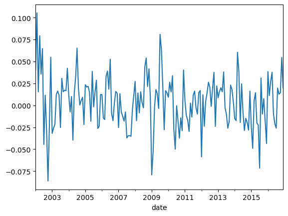
def long_short(X='value', n_groups=10):
    # Assign stocks to groups based on the characteristic X
    df_X['X_group'] = df_X.groupby(['date'])[X].transform(
        lambda x: pd.qcut(x, n_groups, labels=False, duplicates='drop')
    )

    # Calculate equal-weighted portfolio returns for each date and group
    ret_byX = df_X.groupby(['date', 'X_group']).apply(
        lambda x: np.mean(x['re'] + x['rf']), include_groups=False
    ).unstack(level=-1)

    # Construct long-short: long top group, short bottom group
    long_short_ret = ret_byX[n_groups - 1] - ret_byX[0]


    return long_short_ret
long_short(X='value', n_groups=10).plot()
<Axes: xlabel='date'>
9.16. Portfolio formation tradeoffs: Diversification vs Signal Strength#
Why not sort in 100 groups instead on only 10? This way your top portfolio would have much higher average characteristics
Why no simply focus on the stock with the highest characteristic?
Individual stocks have \(\sigma\) = 40 − 80%, so \(\sigma/\sqrt{T}\) makes it nearly impossible to accurately measure E(R). Portfolios have lower \(\sigma\) by diversification.
So you have to trade-off strength of the signal against benefits of diversification
Lets look at this trade-off for Value, Profitability and Momentum
Profitability is simply Gross Profits/Book Assets
Momentum is the cumulative return in the last 12 months skipping the last month (next class!)
def long_short_stats(X='value', n_groups=10):
    r=long_short(X,n_groups)
    return r.std()*12**0.5

for g in [5,10,50,100]:
    print(f'Number of groups: {g}')
    print(long_short_stats('value',g))
    print(long_short_stats('mom',g))
    print(long_short_stats('prof',g))
    print('-------------------')
Number of groups: 5
0.08255392985128295
0.16600364967177128
0.08110923708672288
-------------------
Number of groups: 10
0.10275291207096138
0.2140897671349157
0.11537007514740719
-------------------
Number of groups: 50
0.15912031882198882
0.32389078360187235
0.16863395249433807
-------------------
Number of groups: 100
0.19292759374957436
0.3818200164373193
0.22228821463684753
-------------------
9.17. Things to try#
Look at different characteristics. Which ones create higher spread in average returns
Construct the long-short portfolio that goes long the high portfolio and short the low portfolio. What are the properties of this portfolio?
Which ones have alpha relative to the market in the sample? What do their betas look like?
When they perform poorly?
How correlated are the returns of the long-shorts of different characteristics?
What about interactions of characteristics? How Do you buy “profitable firms” at a good “value” Like Warren likes?
Important:
This is a short sample so things can be done in class quickly
To learn anything meaningful about risk-premiums you would want a longer sample
📝 Key Takeaways
Stacked data frames are the backbone when working with thousands of stocks and multiple characteristics.
Lagged market-cap weights should be the default: they minimize turnover, reflect realistic trading capacity, and eliminate look-ahead bias.
Characteristic-sorted portfolios isolate cross-sectional spreads in the signal; the long-short “top minus bottom” position delivers a clean test of the signal’s pricing power.
Portfolio design choices matter: more groups widen the average-return spread but shrink the number of stocks per bucket; equal-weighting boosts the influence of small caps, while value-weighting is closer to how real money is run.
A single, well-structured function automates experimentation across different signals, making it easy to investigate which characteristics generate higher alpha, when they underperform, and how their long-short returns co-move.
The core tension is signal strength versus diversification: stronger signals often come with higher concentration and trading costs, so practical implementation always balances these forces.