
6. Factor Models#
6.1. 🎯 Learning Objectives#
By the end of this notebook, you will be able to:
Decode the α / β decomposition — Split any asset’s excess return into factor-driven and idiosyncratic pieces
Estimate factor exposure with regression — Use OLS to obtain α, β, and residual statistics
Create tracking and hedged portfolios — Build factor-neutral “portable alpha” positions
Apply risk budgets to position sizing — Determine capital allocation under volatility constraints
Evaluate performance with Sharpe and Appraisal ratios — Distinguish skill from factor exposure
6.2. 📋 Table of Contents#
6.3. 🛠️ Setup #
#@title 🛠️ Setup: Run this cell first (click to expand)

# Core libraries
import numpy as np
import pandas as pd
import matplotlib.pyplot as plt
%matplotlib inline


# Set consistent plot style
plt.style.use('seaborn-v0_8-whitegrid')
plt.rcParams['figure.figsize'] = [10, 6]
plt.rcParams['font.size'] = 12

# Suppress warnings for cleaner output
import warnings
warnings.filterwarnings('ignore')

print("✅ Libraries loaded successfully!")
✅ Libraries loaded successfully!
#@title Helper Function: Get Factor Data
# pandas-datareader: Fetches financial data from various online sources
# We'll use it to get Fama-French factor data from Ken French's website
import datetime
from pandas_datareader.data import DataReader
def get_factors(factors='CAPM', freq='daily'):
    """Download Fama-French factor data.

    Parameters:
    - factors: 'CAPM', 'FF3', 'FF5', or 'FF6'
    - freq: 'daily' or 'monthly'

    Returns: DataFrame with factor returns (as decimals)
    """
    freq_label = '' if freq == 'monthly' else '_' + freq

    if factors == 'CAPM':
        ff = DataReader(f"F-F_Research_Data_Factors{freq_label}", "famafrench", start="1921-01-01")
        df_factor = ff[0][['RF', 'Mkt-RF']]
    elif factors == 'FF3':
        ff = DataReader(f"F-F_Research_Data_Factors{freq_label}", "famafrench", start="1921-01-01")
        df_factor = ff[0][['RF', 'Mkt-RF', 'SMB', 'HML']]
    elif factors == 'FF5':
        ff = DataReader(f"F-F_Research_Data_Factors{freq_label}", "famafrench", start="1921-01-01")
        df_factor = ff[0][['RF', 'Mkt-RF', 'SMB', 'HML']]
        ff2 = DataReader(f"F-F_Research_Data_5_Factors_2x3{freq_label}", "famafrench", start="1921-01-01")
        df_factor = df_factor.merge(ff2[0][['RMW', 'CMA']], on='Date', how='outer')
    else:  # FF6
        ff = DataReader(f"F-F_Research_Data_Factors{freq_label}", "famafrench", start="1921-01-01")
        df_factor = ff[0][['RF', 'Mkt-RF', 'SMB', 'HML']]
        ff2 = DataReader(f"F-F_Research_Data_5_Factors_2x3{freq_label}", "famafrench", start="1921-01-01")
        df_factor = df_factor.merge(ff2[0][['RMW', 'CMA']], on='Date', how='outer')
        ff_mom = DataReader(f"F-F_Momentum_Factor{freq_label}", "famafrench", start="1921-01-01")
        df_factor = df_factor.merge(ff_mom[0], on='Date')
        df_factor.columns = ['RF', 'Mkt-RF', 'SMB', 'HML', 'RMW', 'CMA', 'MOM']

    if freq == 'monthly':
        df_factor.index = pd.to_datetime(df_factor.index.to_timestamp()) + pd.offsets.MonthEnd(0)
    else:
        df_factor.index = pd.to_datetime(df_factor.index)
    return df_factor / 100  # Convert from percent to decimal
6.3.1. Loading Return Data#
# Load excess returns for SPY, WMT, JPM
url = 'https://raw.githubusercontent.com/amoreira2/UG54/refs/heads/main/assets/data/FactorModels_data1.csv'
df_re = pd.read_csv(url, parse_dates=['date'], index_col='date')

print(f"Data range: {df_re.index.min().date()} to {df_re.index.max().date()}")
print(f"Stocks: {list(df_re.columns)}")
# Prepare data (drop missing values)
data = df_re.dropna()
data.tail()
Data range: 1969-03-05 to 2024-12-31
Stocks: ['SPY', 'WMT', 'JPM']
| SPY | WMT | JPM | |
|---|---|---|---|
| date | |||
| 2024-12-24 | 0.010940 | 0.025614 | 0.016269 |
| 2024-12-26 | -0.000106 | 0.001014 | 0.003252 |
| 2024-12-27 | -0.010698 | -0.012349 | -0.008273 |
| 2024-12-30 | -0.011585 | -0.012065 | -0.007844 |
| 2024-12-31 | -0.003811 | -0.002602 | 0.001457 |
6.4. Co-movement #
6.4.1. The Core Insight#
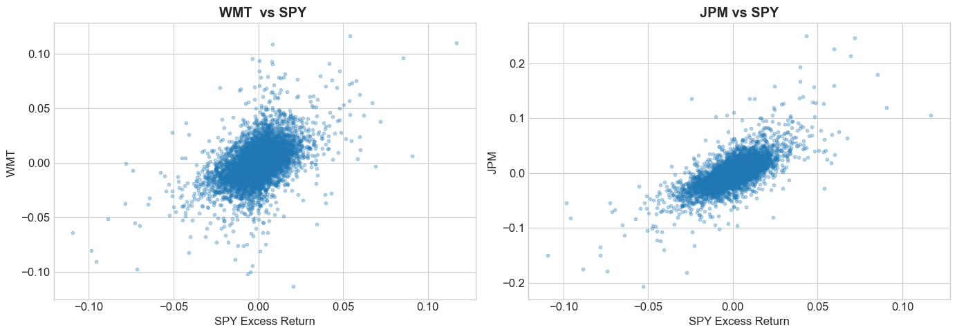
To understand how much to invest in different stocks, the first step is to understand to what extent stocks are alike and to what extent they are different.
It makes no sense to say tht you are buying to buy a bunch of different assets to be diversified if they all behave alike each other
Stocks don’t move independently—they co-move with the market.
But the degree of co-movement varies:
Defensive stocks (utilities, groceries) → less sensitive to market swings
Cyclical stocks (luxury goods, banks) → more sensitive to market swings
High-leverage stocks → particularly vulnerable in downturns
6.4.2. Visualizing Co-movement#
# Create residuals
wmt = data['WMT']
jpm = data['JPM']

# Plot residuals vs factor
fig, axes = plt.subplots(1, 2, figsize=(14, 5))

axes[0].scatter(data['SPY'], wmt, alpha=0.3, s=10)
axes[0].set_xlabel('SPY Excess Return')
axes[0].set_ylabel('WMT ')
axes[0].set_title(f'WMT  vs SPY ', fontweight='bold')

axes[1].scatter(data['SPY'], jpm, alpha=0.3, s=10)
axes[1].set_xlabel('SPY Excess Return')
axes[1].set_ylabel('JPM ')
axes[1].set_title(f'JPM vs SPY', fontweight='bold')

plt.tight_layout()
plt.show()
6.4.3. Towards a Factor Model#
We decompose any asset’s excess return as:
Where:
\(r^e\) = asset’s excess return over risk-free rate
\(\alpha\) = intercept (skill/mispricing)
\(\beta\) = sensitivity to factor
\(f\) = factor excess return (e.g., market)
\(\epsilon\) = idiosyncratic (asset-specific) risk
💡 Key Insight:
This decomposition is always valid—it’s just statistics. The power comes from interpreting each piece:
\(\beta \cdot f\) is the return you could get by investing in the factor in a way that tracks the asset as well as possible
\(\alpha+\epsilon\) is the return specific to the asset only. Alpha is the mean. Epsilon is the noise.
🤔 Think and Code:
How do we estimate \(\beta\) and \(\alpha\) from data?
What should we plot to visualize if the factor model “works”?
What do you expect the correlation between residuals and factor to be?
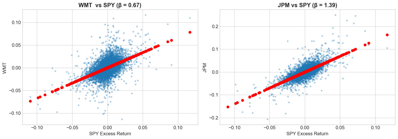
6.4.4. Estimating Beta with Regression#
# statsmodels: Statistical modeling library for Python
# Provides OLS regression, hypothesis testing, and model diagnostics

import statsmodels.formula.api as smf


# Run regressions for WMT and JPM on SPY
model_wmt = smf.ols(formula='WMT ~ SPY', data=data).fit()
model_jpm = smf.ols(formula='JPM ~ SPY', data=data).fit()

alpha_wmt, beta_wmt = model_wmt.params
alpha_jpm, beta_jpm = model_jpm.params

print(f"WMT: α = {alpha_wmt:.6f}, β = {beta_wmt:.3f}")
print(f"JPM: α = {alpha_jpm:.6f}, β = {beta_jpm:.3f}")
WMT: α = 0.000203, β = 0.674
JPM: α = 0.000159, β = 1.395
📌 Remember:
\(\beta < 1\): Less sensitive than market (defensive)
\(\beta = 1\): Same sensitivity as market
\(\beta > 1\): More sensitive than market (aggressive)
6.4.5. Visualizing Co-movement#
# Create residuals
wmt = data['WMT']
jpm = data['JPM']

# Plot residuals vs factor
fig, axes = plt.subplots(1, 2, figsize=(14, 5))

axes[0].scatter(data['SPY'], wmt, alpha=0.3, s=10)
axes[0].scatter(data['SPY'],alpha_wmt+beta_wmt * data['SPY'], color='red', linestyle='-')
axes[0].set_xlabel('SPY Excess Return')
axes[0].set_ylabel('WMT ')
axes[0].set_title(f'WMT  vs SPY (β = {beta_wmt:.2f})', fontweight='bold')

axes[1].scatter(data['SPY'], jpm, alpha=0.3, s=10)
axes[1].scatter(data['SPY'],alpha_jpm+beta_jpm * data['SPY'], color='red', linestyle='-')
axes[1].set_xlabel('SPY Excess Return')
axes[1].set_ylabel('JPM ')
axes[1].set_title(f'JPM vs SPY (β = {beta_jpm:.2f})', fontweight='bold')

plt.tight_layout()
plt.show()

# Verify residuals are uncorrelated with factor
print(f"Correlation of SPY with WMT : {data['SPY'].corr(wmt):.6f}")
print(f"Correlation of SPY with JPM: {data['SPY'].corr(jpm):.6f}")
Correlation of SPY with WMT : 0.492221
Correlation of SPY with JPM: 0.707302
# Create residuals
resid_wmt = data['WMT'] - beta_wmt * data['SPY']
resid_jpm = data['JPM'] - beta_jpm * data['SPY']

# Plot residuals vs factor
fig, axes = plt.subplots(1, 2, figsize=(14, 5))

axes[0].scatter(data['SPY'], resid_wmt, alpha=0.3, s=10)
axes[0].axhline(0, color='red', linestyle='--')
axes[0].set_xlabel('SPY Excess Return')
axes[0].set_ylabel('WMT Residual')
axes[0].set_title(f'WMT Residuals vs SPY (β = {beta_wmt:.2f})', fontweight='bold')

axes[1].scatter(data['SPY'], resid_jpm, alpha=0.3, s=10)
axes[1].axhline(0, color='red', linestyle='--')
axes[1].set_xlabel('SPY Excess Return')
axes[1].set_ylabel('JPM Residual')
axes[1].set_title(f'JPM Residuals vs SPY (β = {beta_jpm:.2f})', fontweight='bold')

plt.tight_layout()
plt.show()

# Verify residuals are uncorrelated with factor
print(f"Correlation of SPY with WMT residuals: {data['SPY'].corr(resid_wmt):.6f}")
print(f"Correlation of SPY with JPM residuals: {data['SPY'].corr(resid_jpm):.6f}")
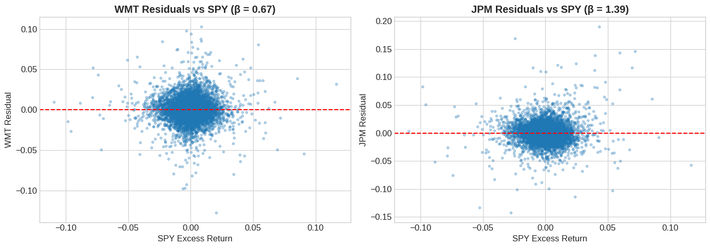
Correlation of SPY with WMT residuals: 0.000000
Correlation of SPY with JPM residuals: 0.000000
6.5. Risk Models vs Expected Return Models #
Factor models serve two distinct purposes:
6.5.1. 👉 Risk Models#
Goal: Explain realized return variation
Assumption: \(\epsilon\) is uncorrelated across assets
Key metric: R-squared (how much variance is explained?)
Can it explain realized returns?
Use case: Risk management, covariance estimation
6.5.2. 👉 Expected Return Models#
Goal: Explain expected return differences
Assumption: \(\alpha = 0\) for all assets
Key metric: Alpha (is it close to zero?)
can it explain differences in Average returns across assets and strategies as a function of factor loadings (i.e. betas?)
Use case: Performance evaluation, asset pricing tests
💡 Key Insight:
A model can be great for risk but poor for expected returns. For stocks, factor models explain lots of variance but still leave substantial uncertainty about expected returns.
6.6. Alpha and Beta: The Organization of Wall Street #
6.6.1. How the Industry is Organized#
The \(\alpha\)- \(\beta\) decomposition is how Wall Street operates:
Big bonuses only come from perceied \(\alpha\) (skill)
Beta exposure is close to a commodity—exact commodity for market exposure, closer to commodity for other factors
Pod shops require traders to be factor-neutral (not only market but across many factors):
6.6.2. From Factor Exposure to Expected Returns#
Taking expectations of our factor model:
Expected return decomposes into:
\(r_f\): Risk-free rate (time value of money)
\(\beta \cdot E[f]\): Premium from factor exposure
\(\alpha\): Abnormal return (skill or mispricing)
⚠️ Caution:
If you have a good model of expected returns, \(\alpha\) should be zero. A significant \(\alpha\) means either:
You found skill/mispricing, OR
Your factor model is missing something
So it is all about interepretation.
In the industry, a trader often takes the factor model as given and try to beat it
The factor model can come from clients or the central book.
If you are a family office, managing money for a sovereign wealth fund, or giving advice to a client it will be your job to determine what factors to include
6.7. Tracking and Hedged Portfolios #
6.7.1. Loading MSFT Data for Hedging Example#
# Load MSFT returns
url_msft = 'https://raw.githubusercontent.com/amoreira2/UG54/refs/heads/main/assets/data/FactorModels_data2.csv'
df_returns = pd.read_csv(url_msft, parse_dates=['date'], index_col='date')

# Get factor data
df_factor = get_factors()

# Align the two DataFrames on common dates
df_returns, df_factor = df_returns.dropna().align(df_factor.dropna(), join='inner', axis=0)

print(f"Data range: {df_returns.index.min().date()} to {df_returns.index.max().date()}")
print(f"Observations: {len(df_returns)}")
Data range: 1986-03-14 to 2024-12-31
Observations: 9778
6.7.2. Running the Factor Regression#
import statsmodels.api as sm

# Compute MSFT excess returns
df_eret = df_returns['MSFT'] - df_factor['RF']

# Prepare regression
X = sm.add_constant(df_factor['Mkt-RF'])  # Add intercept
y = df_eret

# Fit OLS model
model = sm.OLS(y, X).fit()
print(model.summary())
                            OLS Regression Results
==============================================================================
Dep. Variable:                      y   R-squared:                       0.415
Model:                            OLS   Adj. R-squared:                  0.415
Method:                 Least Squares   F-statistic:                     6940.
Date:                Wed, 04 Feb 2026   Prob (F-statistic):               0.00
Time:                        14:10:18   Log-Likelihood:                 26516.
No. Observations:                9778   AIC:                        -5.303e+04
Df Residuals:                    9776   BIC:                        -5.301e+04
Df Model:                           1
Covariance Type:            nonrobust
==============================================================================
                 coef    std err          t      P>|t|      [0.025      0.975]
------------------------------------------------------------------------------
const          0.0006      0.000      3.597      0.000       0.000       0.001
Mkt-RF         1.1876      0.014     83.309      0.000       1.160       1.216
==============================================================================
Omnibus:                     1452.828   Durbin-Watson:                   1.929
Prob(Omnibus):                  0.000   Jarque-Bera (JB):            22202.613
Skew:                           0.141   Prob(JB):                         0.00
Kurtosis:                      10.377   Cond. No.                         87.7
==============================================================================

Notes:
[1] Standard Errors assume that the covariance matrix of the errors is correctly specified.
6.7.3. Magnitudes#
🤔 Think and Code:
Is this alpha economically significant?
What shoudl I do to have a sense of it?
IS it a good bet on a risk-reward sense? What should I look at?
# Extract key statistics
alpha = model.params['const']
beta = model.params['Mkt-RF']
var_r = y.var()
var_f = df_factor['Mkt-RF'].var()
var_e = model.resid.var()
mu_f = df_factor['Mkt-RF'].mean()

print(f"Alpha :     {alpha:.6f}")
print(f"Beta:              {beta:.3f}")
print(f"Variance of MSFT:  {var_r:.6f}")
print(f"Variance of MKT:   {var_f:.6f}")
print(f"Variance of resid: {var_e:.6f}")
print(f"Mean MKT excess:   {mu_f:.6f}")
Alpha :     0.000585
Beta:              1.188
Variance of MSFT:  0.000442
Variance of MKT:   0.000130
Variance of resid: 0.000258
Mean MKT excess:   0.000359
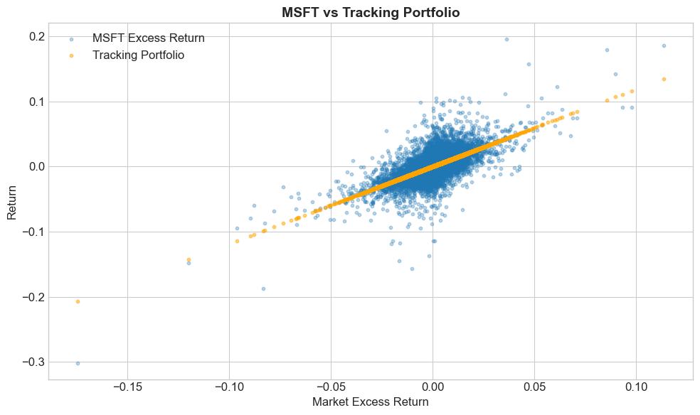
6.7.4. The Tracking Portfolio (also called mimicking portfolio, factor-mimicking portfolio or Hedging Portfolio)#
The tracking portfolio replicates the factor-driven component:
For MSFT with \(\beta \approx 1.2\):
For every 1 dollar in MSFT, hold \(\beta\) dollars in the market factor
# Compute tracking portfolio returns
MKT = df_factor['Mkt-RF']
Portfolio = df_eret
Tracking = MKT * beta

# Plot actual vs tracking
fig, ax = plt.subplots(figsize=(10, 6))
ax.scatter(MKT, Portfolio, alpha=0.3, s=10, label='MSFT Excess Return')
ax.scatter(MKT, Tracking, alpha=0.5, s=10, label='Tracking Portfolio', color='orange')
ax.set_xlabel('Market Excess Return')
ax.set_ylabel('Return')
ax.set_title('MSFT vs Tracking Portfolio', fontsize=14, fontweight='bold')
ax.legend()
plt.tight_layout()
plt.show()
6.7.5. The Hedged Portfolio#
The hedged portfolio removes all factor exposure:
Properties:
Mean return = \(\alpha\) (pure skill)
Volatility = \(\sigma_{\epsilon}\) (only idiosyncratic risk), often that is the compoentn that people call Tracking error
Beta = 0 (by construction, we already stripped out all factor exposure!)
# Compute hedged portfolio
Hedged = Portfolio - Tracking

# Visualize
fig, ax = plt.subplots(figsize=(10, 6))
ax.scatter(MKT, MKT, alpha=0.3, s=10, label='Market (β=1)')
ax.scatter(MKT, Hedged, alpha=0.3, s=10, label='Hedged MSFT (β=0)', color='green')
ax.axhline(0, color='red', linestyle='--', alpha=0.5)
ax.set_xlabel('Market Excess Return')
ax.set_ylabel('Return')
ax.set_title('Hedged Portfolio Has Zero Beta', fontsize=14, fontweight='bold')
ax.legend()
plt.tight_layout()
plt.show()

# Verify
print(f"Hedged portfolio mean (annualized): {Hedged.mean() * 252:.4f}")
print(f"Alpha (annualized):                 {alpha * 252:.4f}")
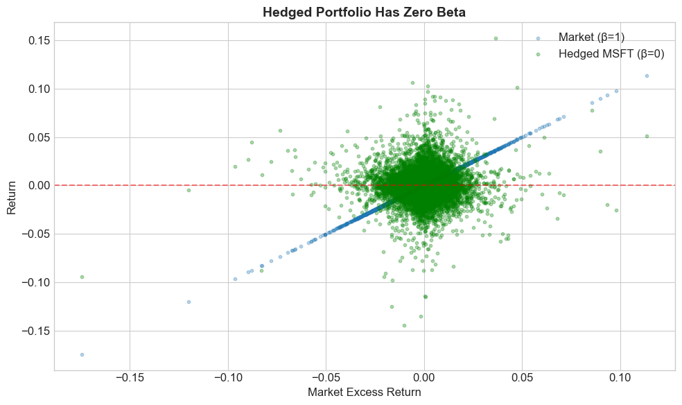
Hedged portfolio mean (annualized): 0.1474
Alpha (annualized):                 0.1474
6.8. Risk Budgets and Position Sizing #
6.8.1. Position Sizing Under a Volatility Budget#
Suppose you have a $1 million/month volatility budget.
How much MSFT can you buy?
What is the math?
# Monthly volatility of MSFT
vol_monthly = np.sqrt(var_r) * np.sqrt(21)  # ~21 trading days per month

# Volatility budget
budget = 1_000_000  # $1M

# Position size
x = ____

print(f"MSFT monthly volatility: {vol_monthly:.4f}")
print(f"Position size: ${x:,.0f}")
---------------------------------------------------------------------------
NameError                                 Traceback (most recent call last)
Cell In[17], line 8
      5 budget = 1_000_000  # $1M
      7 # Position size
----> 8 x = ____
     10 print(f"MSFT monthly volatility: {vol_monthly:.4f}")
     11 print(f"Position size: ${x:,.0f}")

NameError: name '____' is not defined
6.8.2. Expected P&L#
Your expected P&L has two components:
Total: \(x \times (\beta \cdot \mu_f + \alpha) \times 252\)
Risk-adjusted: \(x \times \alpha \times 252\) (what you get paid for)
print(f"Expected annual P&L (total):         ${x * (beta * mu_f + alpha) * 252:,.0f}")
print(f"Expected annual P&L (risk-adjusted): ${x * alpha * 252:,.0f}")
Expected annual P&L (total):         $2,644,594
Expected annual P&L (risk-adjusted): $1,530,371
6.8.3. Hedging Allows Larger Positions#
With hedging, volatility = \(\sigma_\epsilon\) (smaller than \(\sigma_r\)).
You can take a larger position for the same risk budget!
# Hedged volatility (annual)
vol_hedged_annual = np.sqrt(var_e) * np.sqrt(21)

# Annual budget
budget_annual = 1_000_000

# Hedged position size
xe = budget_annual / vol_hedged_annual

print(f"Unhedged vol (annual): {np.sqrt(var_r) * np.sqrt(252):.4f}")
print(f"Hedged vol (annual):   {vol_hedged_annual:.4f}")
print(f"\nUnhedged position: ${x}")
print(f"Hedged position:   ${xe}")
print(f"\nHedged P&L:        ${xe * alpha * 252:,.0f}")
Unhedged vol (annual): 0.3336
Hedged vol (annual):   0.0736
---------------------------------------------------------------------------
NameError                                 Traceback (most recent call last)
Cell In[18], line 12
     10 print(f"Unhedged vol (annual): {np.sqrt(var_r) * np.sqrt(252):.4f}")
     11 print(f"Hedged vol (annual):   {vol_hedged_annual:.4f}")
---> 12 print(f"\nUnhedged position: ${x:,.0f}")
     13 print(f"Hedged position:   ${xe:,.0f}")
     14 print(f"\nHedged P&L:        ${xe * alpha * 252:,.0f}")

NameError: name 'x' is not defined
💡 Key Insight:
Hedging reduces volatility, which allows larger position sizes. If your alpha is genuine, hedging lets you earn more of it!
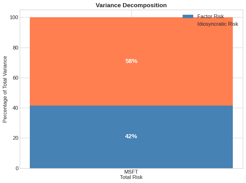
6.10. Variance Decomposition #
6.10.1. Breaking Down Total Risk#
Total variance decomposes into factor and idiosyncratic parts:
The factor risk share is:
# Variance decomposition
factor_var = beta**2 * var_f
idio_var = var_e
total_var = var_r

factor_share = factor_var / total_var
idio_share = idio_var / total_var

print(f"Factor variance contribution: {factor_var:.6f} ({factor_share:.1%})")
print(f"Idiosyncratic variance:       {idio_var:.6f} ({idio_share:.1%})")
print(f"Total variance:               {total_var:.6f}")

# This should equal R-squared
print(f"\nR-squared from regression: {model.rsquared:.3f}")
print(f"Factor share:              {factor_share:.3f}")
Factor variance contribution: 0.000183 (41.5%)
Idiosyncratic variance:       0.000258 (58.5%)
Total variance:               0.000442

R-squared from regression: 0.415
Factor share:              0.415
# Visualize variance decomposition
fig, ax = plt.subplots(figsize=(8, 6))

categories = ['MSFT\nTotal Risk']
factor_vals = [factor_share * 100]
idio_vals = [idio_share * 100]

ax.bar(categories, factor_vals, label='Factor Risk', color='steelblue')
ax.bar(categories, idio_vals, bottom=factor_vals, label='Idiosyncratic Risk', color='coral')

ax.set_ylabel('Percentage of Total Variance')
ax.set_title('Variance Decomposition', fontsize=14, fontweight='bold')
ax.legend()
ax.set_ylim(0, 105)

# Add percentage labels
ax.text(0, factor_share * 50, f'{factor_share:.0%}', ha='center', va='center',
        fontsize=14, fontweight='bold', color='white')
ax.text(0, factor_share * 100 + idio_share * 50, f'{idio_share:.0%}', ha='center',
        va='center', fontsize=14, fontweight='bold', color='white')

plt.tight_layout()
plt.show()
6.11. Exercises #
6.11.1. 🔧 Exercise 1: Estimate Factor Model for JPM#
Using the df_re DataFrame loaded earlier:
Run a regression of JPM excess returns on SPY
Report the \(\alpha\), \(\beta\), and R-squared
Is JPM more or less sensitive to the market than WMT?
💡 Click for solution
import statsmodels.api as sm

# Prepare data
data = df_re.dropna()
X = sm.add_constant(data['SPY'])
y = data['JPM']

# Fit model
model_jpm = sm.OLS(y, X).fit()

print(f"Alpha: {model_jpm.params['const']:.6f}")
print(f"Beta: {model_jpm.params['SPY']:.3f}")
print(f"R-squared: {model_jpm.rsquared:.3f}")
JPM has a higher beta than WMT, making it more sensitive to market movements.
# Your code here
6.11.2. 🔧 Exercise 2: Build a Hedged Portfolio#
Using your JPM regression results:
Compute the hedged portfolio returns: \(r^{\text{hedged}} = r^e_{JPM} - \beta \times r^e_{SPY}\)
Verify that the hedged portfolio has zero correlation with SPY
Calculate the Sharpe ratio of the hedged vs unhedged portfolio
💡 Click for solution
beta_jpm = model_jpm.params['SPY']

# Hedged portfolio
hedged_jpm = data['JPM'] - beta_jpm * data['SPY']

# Verify zero correlation
print(f"Correlation with SPY: {data['SPY'].corr(hedged_jpm):.6f}")

# Sharpe ratios
sharpe_unhedged = (data['JPM'].mean() * 252) / (data['JPM'].std() * np.sqrt(252))
sharpe_hedged = (hedged_jpm.mean() * 252) / (hedged_jpm.std() * np.sqrt(252))

print(f"Sharpe (unhedged): {sharpe_unhedged:.3f}")
print(f"Sharpe (hedged): {sharpe_hedged:.3f}")
# Your code here
6.11.3. 🤔 Exercise 3: Position Sizing Challenge#
You have a $5 million annual volatility budget.
How much can you invest in JPM (unhedged)?
How much can you invest in the hedged JPM strategy?
What is the expected risk-adjusted P&L for each?
💡 Click for solution
budget = 5_000_000

# Volatilities
vol_jpm = data['JPM'].std() * np.sqrt(252)
vol_hedged = hedged_jpm.std() * np.sqrt(252)

# Position sizes
pos_unhedged = budget / vol_jpm
pos_hedged = budget / vol_hedged

print(f"Unhedged position: ${pos_unhedged:,.0f}")
print(f"Hedged position:   ${pos_hedged:,.0f}")

# Risk-adjusted P&L (alpha only)
alpha_jpm = model_jpm.params['const']
pnl_unhedged = pos_unhedged * alpha_jpm * 252
pnl_hedged = pos_hedged * alpha_jpm * 252

print(f"\nRisk-adjusted P&L (unhedged): ${pnl_unhedged:,.0f}")
print(f"Risk-adjusted P&L (hedged):   ${pnl_hedged:,.0f}")
# Your code here
6.12. 📝 Key Takeaways #
Factor models separate what you earn from what you ride. Beta captures common market movements; alpha is the slice of return not explained by those movements.
Hedging out β turns views into “portable” alpha. Going long the asset and short β units of the factor neutralizes systematic risk.
Risk budgets shrink once you hedge intelligently. A hedged position’s lower volatility allows you to deploy more capital for the same risk cap.
Variance decomposition is your monitoring dashboard. It tells you how much of today’s risk is coming from factors versus idiosyncratic shocks.
Tracking portfolios clarify performance attribution. By explicitly matching the factor component, you can assess whether outperformance is genuine skill or hidden beta.
All numbers are frequency-specific. Alpha, variances, and Sharpe ratios must be annualized consistently. Beta is theoretically invariant to frequency.