
To Be Done
import numpy as np
import pandas as pd
%matplotlib inline
import matplotlib.pyplot as plt
import statsmodels.api as sm
C:\Users\alan.moreira\AppData\Roaming\Python\Python39\site-packages\pandas\core\computation\expressions.py:21: UserWarning: Pandas requires version '2.8.4' or newer of 'numexpr' (version '2.8.1' currently installed).
  from pandas.core.computation.check import NUMEXPR_INSTALLED
C:\Users\alan.moreira\AppData\Roaming\Python\Python39\site-packages\pandas\core\arrays\masked.py:60: UserWarning: Pandas requires version '1.3.6' or newer of 'bottleneck' (version '1.3.4' currently installed).
  from pandas.core import (
15. Trading costs and Liquidity#
So we have taken prices as given and discussed quantitative allocation rules that overperform relative to a standard CAPM benchmark.
An important question is whether we would be able to trade at those prices if we tried to implement the strategy.
Liquidity is the ease of trading a security.
This encompass many factors, all of which impose a cost on those wishing to trade.
Sources of illiquidity:
Exogenous transactions costs = brokerage fees, order-processing costs, transaction taxes.
Demand pressure = when need to sell quickly, nautral buyer not available. Whoever is available will ask to be compensated to absorb the trade
Inventory risk = if can’t find a buyer will sell to a market maker who will later sell position. But, since market maker faces future price changes, he might demand compensation for this risk
Private information = concern over trading against an informed party (e.g., insider). Need to be compensated for this risk. Private information can be about fundamentals or about future flows.
Obviuosly a perfect answer to this question requires costly experimentation. It would require trading and measuring how prices change in reponse to your trading behavior.
15.1. Implementation Shortfall#
Wish portfolio: your portfolio is trading costs were zero
Performance of wish portfolio: compute returns in real time assuming you can trade at the mid
Shortfall=return of wish portfolio- return of real portfolio
(after all costs)
Shortfall includes both execution costs ( the costs of trading to get you to the wish portfolio) and opportunity costs ( the costs of deviating from the wish portfolio )
IF you trade quickly what force will increase the Shotfall ?Which will increase?
How should you trade in this world?
Precise answer is highly empirical
But overall shape of the solution is clear
Find size of tracking error that minimize shortfall
IF your weights imply a tracking below the cap, don;t trade
Trade whenever tracking error going above this value
Trade just enough to keep tracking error at the cap
Key for this trade-off is the cost of trading.
Trading cost highly dependent of who is trading
Why?
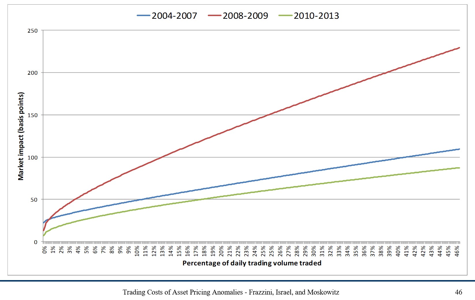
15.2. Absorption capacity#
The idea is to measure how much of the trading volume of each stock you would “use” to implement the strategy for a given position size
Specifically:
The idea is that if you trade a small share of the volume, you are likely to be able to trade at the posted prices.
This graph below shows costs for Trades made by AQR
15.3. How much do you actually need to trade?#
To compute how much you need to trade you need to compare the desired weights in date \(t\) with the weights you have in the end of date \(t+1\).
Before trading, your weight in date \(t+1\) is
If the desired position in the stock is \(w_{i,t+1}^*\), then $\( \begin{align} UsedVolume_{i,t}&=\frac{position \times \bigg(w_{i,t+1}^*-w_{i,t+1}(\text{before trading})\bigg)}{Volume_{i,t}} \\ &=\frac{position}{Volume_{i,t}}\left(w_{i,t+1}^*-\frac{w_{i,t}^*(1+r_{i,t+1})}{1+r_{t+1}^{strategy}}\right) \end{align}\)$
\(UsedVolume_{i,t}\) is a stock-time specific statistic. Implementability will depend on how high this quantity is across time and across stocks– the lower the better.
If it is very high (i.e., close to 1), it means that your position would require almost all volume in a particular stock. It doesn’t mean that you wouldn’t be able to trade, but likely prices would move against you (i.e., go up as you buy, do down as you sell)
One very conservative way of looking at it is to look at the maximum of this statistic across stocks. This tells you the “weakest” link in your portfolio formation.
The max statistic is the right one to look at if you are unwilling to deviate from your “wish portfolio”.
But the “wish portfolio” does not take into account transaction costs
How can portfolios take into account trading costs to reduce total costs substantially?
Can we change the portfolios to reduce trading costs without altering them significantly?
One simple way of looking at this is to look at the 95/75/50 percentiles of the used volume distribution.
If it declines steeply it might make sense to avoid the 5% to 25% of the stocks that are least liquid in you portfolio
But as you deviate from the original portfolio you will have tracking error relative to the original strategy.
crsp=pd.read_pickle('https://github.com/amoreira2/Fin418/blob/main/assets/data/crspm2005_2020.pkl?raw=true')
from pandas.tseries.offsets import *

# change variable format to int
crsp[['permno']]=crsp[['permno']].astype(int)
# Line up date to be end of month
crsp['date']=crsp['date']+MonthEnd(0)

# calculate market equity
# why do we use absolute value of price?
crsp['me']=crsp['prc'].abs()*crsp['shrout']
# drop price and shareoustandng since we won't need it anymore

crsp=crsp[['permno','date','ret', 'me','vol','prc']].sort_values(['permno','date']).set_index('date').drop_duplicates().reset_index()
crsp
| date | permno | ret | me | vol | prc | |
|---|---|---|---|---|---|---|
| 0 | 2005-01-31 | 10001 | -0.040580 | 1.717890e+04 | 515.0 | 6.620000 |
| 1 | 2005-02-28 | 10001 | -0.045166 | 1.642828e+04 | 726.0 | 6.321000 |
| 2 | 2005-03-31 | 10001 | 0.124822 | 1.866375e+04 | 4107.0 | 7.110000 |
| 3 | 2005-04-30 | 10001 | -0.074684 | 1.726987e+04 | 527.0 | 6.579000 |
| 4 | 2005-05-31 | 10001 | 0.219030 | 2.105250e+04 | 1990.0 | 8.020000 |
| ... | ... | ... | ... | ... | ... | ... |
| 763616 | 2020-08-31 | 93436 | 0.741452 | 4.643391e+08 | 4051970.0 | 498.320007 |
| 763617 | 2020-09-30 | 93436 | -0.139087 | 4.067015e+08 | 17331954.0 | 429.010010 |
| 763618 | 2020-10-31 | 93436 | -0.095499 | 3.678235e+08 | 8330610.0 | 388.040009 |
| 763619 | 2020-11-30 | 93436 | 0.462736 | 5.380286e+08 | 7811501.0 | 567.599976 |
| 763620 | 2020-12-31 | 93436 | 0.243252 | 6.689053e+08 | 11962716.0 | 705.669983 |
763621 rows × 6 columns
# data=crsp_m.copy()
# ngroups=10

def momreturns_w(data, ngroups):

    # step1. create a temporary crsp dataset
    _tmp_crsp = data[['permno','date','ret', 'me','vol','prc']].sort_values(['permno','date']).set_index('date').drop_duplicates()
    _tmp_crsp['volume']=_tmp_crsp['vol']*_tmp_crsp['prc'].abs()*100/1e6 # in million dollars like me

    # step 2: construct the signal
    _tmp_crsp['grossret']=_tmp_crsp['ret']+1
    _tmp_cumret=_tmp_crsp.groupby('permno')['grossret'].rolling(window=12).apply(np.prod, raw=True)-1
    _tmp_cumret=_tmp_cumret.reset_index().rename(columns={'grossret':'cumret'})

    _tmp = pd.merge(_tmp_crsp.reset_index(), _tmp_cumret[['permno','date','cumret']], how='left', on=['permno','date'])
    # merge the 12 month return signal back to the original database
    _tmp['mom']=_tmp.groupby('permno')['cumret'].shift(2)

    # step 3: rank assets by signal
    mom=_tmp.sort_values(['date','permno']) # sort by date and firm identifier
    mom=mom.dropna(subset=['mom'], how='any')# drop the row if any of these variables 'mom','ret','me' are missing
    mom['mom_group']=mom.groupby(['date'])['mom'].transform(lambda x: pd.qcut(x, ngroups, labels=False,duplicates='drop'))
    # create `ngroups` groups each month. Assign membership accroding to the stock ranking in the distribution of trading signal
    # in a given month
    # transform in string the group names
    mom=mom.dropna(subset=['mom_group'], how='any')# drop the row if any of 'mom_group' is missing
    mom['mom_group']=mom['mom_group'].astype(int).astype(str).apply(lambda x: 'm{}'.format(x))

    mom['date']=mom['date']+MonthEnd(0) #shift all the date to end of the month
    mom=mom.sort_values(['permno','date']) # resort

    # step 4: form portfolio weights
    def wavg_wght(group, ret_name, weight_name):
        d = group[ret_name]
        w = group[weight_name]
        try:
            group['Wght']=(w) / w.sum()
            return group[['permno','Wght']]
        except ZeroDivisionError:
            return np.nan
    # We now simply have to  use the above function to construct the portfolio

    # the code below applies the function in each date,mom_group group,
    # so it applies the function to each of these subgroups of the data set,
    # so it retursn one time-series for each mom_group, as it average the returns of
    # all the firms in a given group in a given date

    weights = mom.groupby(['date','mom_group']).apply(wavg_wght, 'ret','me')

    # merge back
    weights=mom.merge(weights,on=['date','permno'])
    weights=weights.sort_values(['date','permno'])

    weights['mom_group_lead']=weights.groupby('permno').mom_group.shift(-1)
    weights['Wght_lead']=weights.groupby('permno').Wght.shift(-1)
    weights=weights.sort_values(['permno','date'])

    def wavg_ret(group, ret_name, weight_name):
        d = group[ret_name]
        w = group[weight_name]
        try:
            return (d * w).sum() / w.sum()
        except ZeroDivisionError:
            return np.nan

    port_vwret = weights.groupby(['date','mom_group']).apply(wavg_ret, 'ret','Wght')
    port_vwret = port_vwret.reset_index().rename(columns={0:'port_vwret'})# give a name to the new time-seires


    weights=weights.merge(port_vwret,how='left',on=['date','mom_group'])

    port_vwret=port_vwret.set_index(['date','mom_group']) # set indexes
    port_vwret=port_vwret.unstack(level=-1) # unstack so we have in each column the different portfolios, and in each
    port_vwret=port_vwret.port_vwret

    return port_vwret, weights
port_ret, wght=momreturns_w(crsp, 10)
C:\Users\alan.moreira\AppData\Local\Temp\ipykernel_1440\3351365901.py:48: DeprecationWarning: DataFrameGroupBy.apply operated on the grouping columns. This behavior is deprecated, and in a future version of pandas the grouping columns will be excluded from the operation. Either pass `include_groups=False` to exclude the groupings or explicitly select the grouping columns after groupby to silence this warning.
  weights = mom.groupby(['date','mom_group']).apply(wavg_wght, 'ret','me')
---------------------------------------------------------------------------
ValueError                                Traceback (most recent call last)
Input In [4], in <cell line: 1>()
----> 1 port_ret, wght=momreturns_w(crsp, 10)

Input In [3], in momreturns_w(data, ngroups)
     48 weights = mom.groupby(['date','mom_group']).apply(wavg_wght, 'ret','me')
     50 # merge back
---> 51 weights=mom.merge(weights,on=['date','permno'])
     52 weights=weights.sort_values(['date','permno'])
     54 weights['mom_group_lead']=weights.groupby('permno').mom_group.shift(-1)

File ~\AppData\Roaming\Python\Python39\site-packages\pandas\core\frame.py:10819, in DataFrame.merge(self, right, how, on, left_on, right_on, left_index, right_index, sort, suffixes, copy, indicator, validate)
  10800 @Substitution("")
  10801 @Appender(_merge_doc, indents=2)
  10802 def merge(
   (...)
  10815     validate: MergeValidate | None = None,
  10816 ) -> DataFrame:
  10817     from pandas.core.reshape.merge import merge
> 10819     return merge(
  10820         self,
  10821         right,
  10822         how=how,
  10823         on=on,
  10824         left_on=left_on,
  10825         right_on=right_on,
  10826         left_index=left_index,
  10827         right_index=right_index,
  10828         sort=sort,
  10829         suffixes=suffixes,
  10830         copy=copy,
  10831         indicator=indicator,
  10832         validate=validate,
  10833     )

File ~\AppData\Roaming\Python\Python39\site-packages\pandas\core\reshape\merge.py:170, in merge(left, right, how, on, left_on, right_on, left_index, right_index, sort, suffixes, copy, indicator, validate)
    155     return _cross_merge(
    156         left_df,
    157         right_df,
   (...)
    167         copy=copy,
    168     )
    169 else:
--> 170     op = _MergeOperation(
    171         left_df,
    172         right_df,
    173         how=how,
    174         on=on,
    175         left_on=left_on,
    176         right_on=right_on,
    177         left_index=left_index,
    178         right_index=right_index,
    179         sort=sort,
    180         suffixes=suffixes,
    181         indicator=indicator,
    182         validate=validate,
    183     )
    184     return op.get_result(copy=copy)

File ~\AppData\Roaming\Python\Python39\site-packages\pandas\core\reshape\merge.py:794, in _MergeOperation.__init__(self, left, right, how, on, left_on, right_on, left_index, right_index, sort, suffixes, indicator, validate)
    784     raise MergeError(msg)
    786 self.left_on, self.right_on = self._validate_left_right_on(left_on, right_on)
    788 (
    789     self.left_join_keys,
    790     self.right_join_keys,
    791     self.join_names,
    792     left_drop,
    793     right_drop,
--> 794 ) = self._get_merge_keys()
    796 if left_drop:
    797     self.left = self.left._drop_labels_or_levels(left_drop)

File ~\AppData\Roaming\Python\Python39\site-packages\pandas\core\reshape\merge.py:1297, in _MergeOperation._get_merge_keys(self)
   1295 rk = cast(Hashable, rk)
   1296 if rk is not None:
-> 1297     right_keys.append(right._get_label_or_level_values(rk))
   1298 else:
   1299     # work-around for merge_asof(right_index=True)
   1300     right_keys.append(right.index._values)

File ~\AppData\Roaming\Python\Python39\site-packages\pandas\core\generic.py:1905, in NDFrame._get_label_or_level_values(self, key, axis)
   1902 other_axes = [ax for ax in range(self._AXIS_LEN) if ax != axis]
   1904 if self._is_label_reference(key, axis=axis):
-> 1905     self._check_label_or_level_ambiguity(key, axis=axis)
   1906     values = self.xs(key, axis=other_axes[0])._values
   1907 elif self._is_level_reference(key, axis=axis):

File ~\AppData\Roaming\Python\Python39\site-packages\pandas\core\generic.py:1867, in NDFrame._check_label_or_level_ambiguity(self, key, axis)
   1859 label_article, label_type = (
   1860     ("a", "column") if axis_int == 0 else ("an", "index")
   1861 )
   1863 msg = (
   1864     f"'{key}' is both {level_article} {level_type} level and "
   1865     f"{label_article} {label_type} label, which is ambiguous."
   1866 )
-> 1867 raise ValueError(msg)

ValueError: 'date' is both an index level and a column label, which is ambiguous.
wght.head()
| date | permno | ret | me | vol | prc | volume | grossret | cumret | mom | mom_group | Wght | mom_group_lead | Wght_lead | port_vwret | |
|---|---|---|---|---|---|---|---|---|---|---|---|---|---|---|---|
| 0 | 2006-02-28 | 10001 | -0.010537 | 27522.091006 | 439.0 | 9.390 | 0.412221 | 0.989463 | 0.499266 | 0.411365 | m8 | 0.000016 | m8 | 0.000024 | -0.003999 |
| 1 | 2006-03-31 | 10001 | 0.170394 | 32222.679329 | 777.0 | 10.990 | 0.853923 | 1.170394 | 0.560008 | 0.446795 | m8 | 0.000024 | m8 | 0.000020 | 0.032930 |
| 2 | 2006-04-30 | 10001 | -0.094631 | 29173.399441 | 883.0 | 9.950 | 0.878585 | 0.905369 | 0.526377 | 0.499266 | m8 | 0.000020 | m8 | 0.000024 | 0.018943 |
| 3 | 2006-05-31 | 10001 | -0.010452 | 28633.911396 | 319.0 | 9.766 | 0.311535 | 0.989548 | 0.239037 | 0.560008 | m8 | 0.000024 | m7 | 0.000023 | -0.046612 |
| 4 | 2006-06-30 | 10001 | -0.076387 | 26464.681343 | 1186.0 | 9.020 | 1.069772 | 0.923613 | 0.014145 | 0.526377 | m7 | 0.000023 | m6 | 0.000017 | 0.001877 |
# construct dollars of each stock that need to be bought (sold) at date t+1
mom=wght.copy()
mom['trade']=(mom.Wght_lead*(mom.mom_group==mom.mom_group_lead)-mom.Wght*(1+mom.ret)/(1+mom.port_vwret))
mom['trade_newbuys']=(~(mom.mom_group==mom.mom_group_lead))*mom.Wght_lead
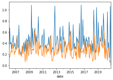
# per dollar of position how much do you have to trade every month?
mom.groupby(['date','mom_group']).trade.apply(lambda x:x.abs().sum()).loc[:,'m9'].plot()
mom.groupby(['date','mom_group_lead']).trade_newbuys.apply(lambda x:x.abs().sum()).loc[:,'m9'].plot()
<AxesSubplot:xlabel='date'>
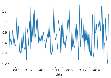
total_trade=mom.groupby(['date','mom_group']).trade.apply(lambda x:x.abs().sum()).loc[:,'m9']+mom.groupby(['date','mom_group_lead']).trade_newbuys.apply(lambda x:x.abs().sum()).loc[:,'m9']

total_trade.plot()
<AxesSubplot:xlabel='date'>
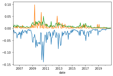
# lets look at the most illiquid stocks, the stocks that I will likely have most trouble trading
# lets start by normalizing the amount of trade per stock volume

mom['tradepervol']=mom.trade/mom.volume

mom['trade_newbuyspervol']=mom.trade_newbuys/mom.volume
# this allow us to study how much of the volume of each stock I will be "using"
# lets choose a position size, here in millions of dollars , because that is the normalization we used for the volume data
Position=1e3 #(1e3 means one billion dollars)
threshold=0.05
(Position*(mom.groupby(['date','mom_group']).tradepervol.quantile(threshold).loc[:,'m9'])).plot()
(Position*(mom.groupby(['date','mom_group']).tradepervol.quantile(1-threshold).loc[:,'m9'])).plot()

(Position*(mom.groupby(['date','mom_group']).trade_newbuyspervol.quantile(1-threshold).loc[:,'m9'])).plot()
<AxesSubplot:xlabel='date'>
Tracking error
Let $\(W^{wishportfolio}_t\)\( and \)\(W^{Implementationportfolio}_t\)$ weights , then consider the following regression
a good implementation portfolio has \(\beta=1\) and \(\sigma(\epsilon)\) and \(\alpha\approx 0\).
So one can think of \(|\beta-1|\), \(\sigma(\epsilon)\) , and \(\alpha\) as three dimensions of tracking error.
The \(\beta\) dimension can be more easily correted by levering up and down the tracking portoflio (of possible)
The \(\sigma(\epsilon)\) can only be corrected by simply making the implemenetation portoflio more similar to the wish portfolio. The cost of this is not obvious. Really depends how this tracking error relates to other stuff in your portfolio.
\(\alpha\) is the important part. The actual cost that you expect to pay to deviate from the wish portfolio
In the industry people typicall refer to tracking error as simply
The volatility of a portfolio that goes long the implementation portfolio and shorts the wish portfolio.
This mixes together \(|\beta-1|\), \(\sigma(\epsilon)\) and completely ignores \(\alpha\)
In the end the Implementation portfolio is chosen by trading off trading costs (market impact) and opportunity cost (tracking error).
So you can simply construct strategies that avoid these 5% less liquid stocks, and see how much your tracking error increases and whether these tracking errors are worth the reduction in trading costs
How to construct an Implementation portfolio?
A simple strategy: weight by trading volume -> this make sure that you use the same amount of trading volume across all your positions
Harder to implement: do not buy stocks that are illiquid now or likely to be illiquid next period. Amounts to add another signal interected to the momentum signal. Only buy if illiquid signal not too strong.
How to change our code to implement the volume-weighted approach?
def momreturns(data, ngroups,wghtvar='me'):

    # step1. create a temporary crsp dataset
    _tmp_crsp = data[['permno','date','ret', 'me','vol','prc']].sort_values(['permno','date']).set_index('date').drop_duplicates()
    _tmp_crsp['volume']=_tmp_crsp['vol']*_tmp_crsp['prc'].abs()*100/1e6 # in million dollars like me

    # step 2: construct the signal
    _tmp_crsp['grossret']=_tmp_crsp['ret']+1
    _tmp_cumret=_tmp_crsp.groupby('permno')['grossret'].rolling(window=12).apply(np.prod, raw=True)-1
    _tmp_cumret=_tmp_cumret.reset_index().rename(columns={'grossret':'cumret'})

    _tmp = pd.merge(_tmp_crsp.reset_index(), _tmp_cumret[['permno','date','cumret']], how='left', on=['permno','date'])
    # merge the 12 month return signal back to the original database
    _tmp['mom']=_tmp.groupby('permno')['cumret'].shift(2)

    # step 3: rank assets by signal
    mom=_tmp.sort_values(['date','permno']) # sort by date and firm identifier
    mom=mom.dropna(subset=['mom'], how='any')# drop the row if any of these variables 'mom','ret','me' are missing
    mom['mom_group']=mom.groupby(['date'])['mom'].transform(lambda x: pd.qcut(x, ngroups, labels=False,duplicates='drop'))
    # create `ngroups` groups each month. Assign membership accroding to the stock ranking in the distribution of trading signal
    # in a given month
    # transform in string the group names
    mom=mom.dropna(subset=['mom_group'], how='any')# drop the row if any of 'mom_group' is missing
    mom['mom_group']=mom['mom_group'].astype(int).astype(str).apply(lambda x: 'm{}'.format(x))

    mom['date']=mom['date']+MonthEnd(0) #shift all the date to end of the month
    mom=mom.sort_values(['permno','date']) # resort

    # step 4: form portfolio weights
    def wavg_wght(group, ret_name, weight_name):
        d = group[ret_name]
        w = group[weight_name]
        try:
            group['Wght']=(w) / w.sum()
            return group[['permno','Wght']]
        except ZeroDivisionError:
            return np.nan
    # We now simply have to  use the above function to construct the portfolio

    # the code below applies the function in each date,mom_group group,
    # so it applies the function to each of these subgroups of the data set,
    # so it retursn one time-series for each mom_group, as it average the returns of
    # all the firms in a given group in a given date

    weights = mom.groupby(['date','mom_group']).apply(wavg_wght, 'ret',wghtvar)

    # merge back
    weights=mom.merge(weights,on=['date','permno'])
    weights=weights.sort_values(['date','permno'])

    weights['mom_group_lead']=weights.groupby('permno').mom_group.shift(-1)
    weights['Wght_lead']=weights.groupby('permno').Wght.shift(-1)
    weights=weights.sort_values(['permno','date'])

    def wavg_ret(group, ret_name, weight_name):
        d = group[ret_name]
        w = group[weight_name]
        try:
            return (d * w).sum() / w.sum()
        except ZeroDivisionError:
            return np.nan

    port_vwret = weights.groupby(['date','mom_group']).apply(wavg_ret, 'ret','Wght')
    port_vwret = port_vwret.reset_index().rename(columns={0:'port_vwret'})# give a name to the new time-seires


    weights=weights.merge(port_vwret,how='left',on=['date','mom_group'])

    port_vwret=port_vwret.set_index(['date','mom_group']) # set indexes
    port_vwret=port_vwret.unstack(level=-1) # unstack so we have in each column the different portfolios, and in each
    port_vwret=port_vwret.port_vwret

    return port_vwret, weights
momportfoliosme,wght=momreturns(crsp,10,wghtvar='me')
momportfoliosvol,wght_vol=momreturns(crsp,10,wghtvar='vol')
momportfolios=momportfoliosme.merge(momportfoliosvol,left_index=True,right_index=True,suffixes=['_me','_vol'])
momportfolios[['m9_me','m9_vol']].plot()
<AxesSubplot:xlabel='date'>
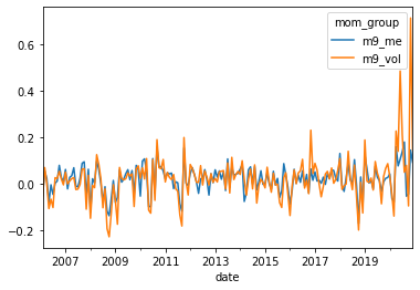
Is this good how do you compare?
Look at tracking error
Don’t be fooled by the long-only performance–replciating the market is easy!
# lets look at it's tracking error
y=momportfolios['m9_vol']
x=momportfolios['m9_me']
x=sm.add_constant(x)
results = sm.OLS(y,x).fit()
results.summary()
| Dep. Variable: | m9_vol | R-squared: | 0.611 |
|---|---|---|---|
| Model: | OLS | Adj. R-squared: | 0.609 |
| Method: | Least Squares | F-statistic: | 277.7 |
| Date: | Wed, 01 May 2024 | Prob (F-statistic): | 4.18e-38 |
| Time: | 17:39:33 | Log-Likelihood: | 242.81 |
| No. Observations: | 179 | AIC: | -481.6 |
| Df Residuals: | 177 | BIC: | -475.2 |
| Df Model: | 1 | ||
| Covariance Type: | nonrobust |
| coef | std err | t | P>|t| | [0.025 | 0.975] | |
|---|---|---|---|---|---|---|
| const | -0.0050 | 0.005 | -1.020 | 0.309 | -0.015 | 0.005 |
| m9_me | 1.3036 | 0.078 | 16.664 | 0.000 | 1.149 | 1.458 |
| Omnibus: | 207.284 | Durbin-Watson: | 1.986 |
|---|---|---|---|
| Prob(Omnibus): | 0.000 | Jarque-Bera (JB): | 8869.659 |
| Skew: | 4.469 | Prob(JB): | 0.00 |
| Kurtosis: | 36.307 | Cond. No. | 16.7 |
Notes:
[1] Standard Errors assume that the covariance matrix of the errors is correctly specified.
Observations:
The beta difference can be adjusted by taking a smaller position on the implementation portfolio
The alpha is the actual tracking error loss. How much you expect to loose.
One calculation that people do is to see how much you are getting for your momentum exposure
[momportfolios['m9_vol'].mean()/results.params[1]*12,momportfolios['m9_me'].mean()*12]
[0.17998714127139948, 0.2261181726535535]
But be careful to not over interpret this. We are working today with a very short sample, less than 20 years, for average returns tests that is not much at all.
But beta/residulas are well measured even in fairly short samples.
In addition to that you also have to eat the strategy residual risk
[results.resid.std(),momportfolios['m9_me'].std()]
[0.06249878812223737, 0.06005053427493518]
It is sizable, about the level of the original strategy volatility
How our implemented strategy compare with the desired strategy?
df=pd.read_pickle('https://raw.githubusercontent.com/amoreira2/Fin418/main/assets/data/df_WarrenBAndCathieW_monthly.pkl')
Factors=df.drop(['BRK','ARKK','RF'],axis=1)
Factors = Factors.rename(columns={Factors.columns[-1]: 'Mom'})

Factors.mean()*12
Mkt-RF    0.100955
SMB       0.012654
HML       0.011914
RMW       0.041875
CMA       0.012701
Mom       0.069910
dtype: float64
portfolios=momportfolios.merge(Factors,left_index=True,right_index=True)
portfolios.head()
| m0_me | m1_me | m2_me | m3_me | m4_me | m5_me | m6_me | m7_me | m8_me | m9_me | ... | m6_vol | m7_vol | m8_vol | m9_vol | Mkt-RF | SMB | HML | RMW | CMA | Mom | |
|---|---|---|---|---|---|---|---|---|---|---|---|---|---|---|---|---|---|---|---|---|---|
| 2006-02-28 | -0.012354 | -0.006109 | 0.012724 | 0.017131 | 0.012390 | 0.014931 | 0.008770 | 0.008683 | -0.003999 | -0.051872 | ... | 0.016308 | 0.012868 | -0.016740 | -0.064788 | -0.0030 | -0.0042 | -0.0034 | -0.0051 | 0.0191 | -0.0184 |
| 2006-03-31 | 0.043584 | 0.029708 | 0.034453 | 0.012203 | 0.013299 | 0.005424 | 0.014716 | 0.026616 | 0.032930 | 0.054823 | ... | 0.023306 | 0.102972 | 0.149737 | 0.069339 | 0.0146 | 0.0338 | 0.0060 | 0.0006 | -0.0041 | 0.0126 |
| 2006-05-31 | -0.026365 | -0.024219 | 0.001555 | -0.015647 | -0.030534 | -0.027217 | -0.032916 | -0.031146 | -0.046612 | -0.080706 | ... | -0.058780 | -0.056930 | -0.079337 | -0.107404 | -0.0357 | -0.0285 | 0.0241 | 0.0115 | 0.0146 | -0.0370 |
| 2006-06-30 | -0.029358 | 0.006137 | -0.002789 | 0.002618 | 0.004338 | 0.002428 | 0.011803 | 0.001877 | 0.023077 | -0.005062 | ... | -0.019315 | -0.004445 | 0.013017 | -0.067229 | -0.0035 | -0.0024 | 0.0085 | 0.0132 | -0.0007 | 0.0154 |
| 2006-07-31 | -0.058296 | -0.036734 | 0.022658 | -0.005353 | 0.024988 | 0.010822 | 0.005927 | -0.008269 | -0.022406 | -0.046551 | ... | -0.008441 | -0.033398 | -0.040144 | -0.102966 | -0.0078 | -0.0363 | 0.0260 | 0.0163 | 0.0090 | -0.0212 |
5 rows × 26 columns
# things to look at:

#y=portfolios['m9_me']
#y=momportfolios['m9_vol']
#y=momportfolios['m9_me']-momportfolios['m0_me']


y=portfolios['m9_me']-portfolios['m0_me']
x=portfolios['Mom']
x=sm.add_constant(x)
results = sm.OLS(y,x).fit()
results.summary()
| Dep. Variable: | y | R-squared: | 0.645 |
|---|---|---|---|
| Model: | OLS | Adj. R-squared: | 0.643 |
| Method: | Least Squares | F-statistic: | 227.5 |
| Date: | Wed, 01 May 2024 | Prob (F-statistic): | 6.34e-30 |
| Time: | 17:46:46 | Log-Likelihood: | 150.75 |
| No. Observations: | 127 | AIC: | -297.5 |
| Df Residuals: | 125 | BIC: | -291.8 |
| Df Model: | 1 | ||
| Covariance Type: | nonrobust |
| coef | std err | t | P>|t| | [0.025 | 0.975] | |
|---|---|---|---|---|---|---|
| const | -0.0231 | 0.007 | -3.504 | 0.001 | -0.036 | -0.010 |
| Mom | 1.9579 | 0.130 | 15.085 | 0.000 | 1.701 | 2.215 |
| Omnibus: | 93.627 | Durbin-Watson: | 2.091 |
|---|---|---|---|
| Prob(Omnibus): | 0.000 | Jarque-Bera (JB): | 691.904 |
| Skew: | -2.555 | Prob(JB): | 5.69e-151 |
| Kurtosis: | 13.229 | Cond. No. | 19.7 |
Notes:
[1] Standard Errors assume that the covariance matrix of the errors is correctly specified.
why such a large difference even for the strategy that follows the Momentum strategy?